- 1 Introduction
- 2 Installation
- 2.1 System Requirements
- 2.2 Software Installation
- 2.3 Configuring Python Scripting Support
- 2.4 Configuring the IBM Rational DOORS Integration
- 2.5 Uninstall INCHRON Tool-Suite
- 2.6 Re-install INCHRON Tool-Suite
- 3 Basics
- 4 Projects
- 5 Online Help
- 6 System Modeling
- 6.1 Modules
- 6.2 Module System
- 6.2.1 Concept of Module System
- 6.2.2 Adding and Removing System Elements
- 6.2.3 Drag & Drop and Copy & Paste
- 6.2.4 Project Information
- 6.2.5 Compiler And Preprocessor Options
- 6.2.6 Microprocessors
- 6.2.7 Peripheral Components
- 6.2.8 Add Source Files
- 6.2.9 Scheduler
- 6.2.10 Defining Processes
- 6.2.11 Modeling AUTOSAR Runnables
- 6.2.12 Modeling Process Dependencies
- 6.2.13 Event Chains
- 6.2.14 Rest Bus Model
- 6.3 Module Architecture
- 6.4 Module Execution Time
- 6.5 Module Clocks
- 6.6 Module Requirements
- 6.6.1 Concept of Module Requirements
- 6.6.2 Requirement Types
- 6.6.3 Process Net Execution Time Requirement
- 6.6.4 Event Net Execution Time Requirement
- 6.6.5 Net Slack Time Requirement
- 6.6.6 Response Time Requirement
- 6.6.7 Event Timing Requirement
- 6.6.8 Illegal Event Requirement
- 6.6.9 RTOS Failure Requirement
- 6.6.10 Event Periodicity Requirement
- 6.6.11 Load Requirement
- 6.6.12 Event Chain Timing Requirement
- 6.6.13 Import and Export of Requirements
- 6.7 Module Stimulation
- 6.7.1 Concept of Module Stimulation
- 6.7.2 Defining a Stimulation Scenario
- 6.7.2.1 Stimulation Scenario Parameters
- 6.7.2.2 Stimulation Generators
- 6.7.2.3 Selecting the Target
- 6.7.2.4 Configuring the Stimulation Generator
- 6.7.2.5 Stimulation Parameters - Disturbance
- 6.7.2.6 Stimulation Parameters - Drift
- 6.7.2.7 Limiting Stimulations with a Burst Filter
- 6.7.2.8 Stimulation Preview
- 6.7.3 Composite Scenario
- 6.7.4 Import and Export of Scenarios
- 7 Simulation
- 7.1 The Simulation Concept
- 7.2 Running a Simulation
- 7.3 Automatic Breakpoints
- 7.4 Environment Variables
- 7.5 Stimulation
- 7.6 Real-Time Requirements
- 7.7 Visualization
- 7.7.1 Time Range Filter
- 7.7.2 View Profiles
- 7.7.3 Statistics View
- 7.7.4 Diagram Types
- 7.7.5 x/t Diagrams
- 7.7.6 Diagram Usage
- 7.7.7 State Diagram
- 7.7.8 Gantt Diagram
- 7.7.9 Sequence Diagram
- 7.7.10 Event Chain Diagram
- 7.7.11 Histogram
- 7.7.12 Box Plot Diagram
- 7.7.13 Load Diagram
- 7.7.14 Stack Diagram
- 7.7.15 Event Diagrams
- 7.7.16 Nesting Diagram
- 7.7.17 Console View
- 7.8 Saving and Loading Trace Files
- 7.9 Export of Stimulation Scenarios
- 7.10 Reporting
- 8 Validation
- 9 Optimization
- 10 Interactive Design of Dynamic Architectures
- 11 Integration with IBM Rational Software
- 12 Subversion Integration
- A Technical Data
- A.1 Target Systems
- A.2 Load Calculation
- A.3 INCHRON Tool-Suite File Formats
- A.3.1 File Format of INCHRON Projects
- A.3.2 File Format of INCHRON Target Models
- A.3.3 File Format of Stimulation Scenarios
- A.3.4 File Format of Requirements
- A.3.5 File Format of View Profiles
- A.3.6 File Formats for Stimulation Data
- A.3.7 File Formats for Simulation Traces
- A.3.8 File Format for Reports
- A.3.9 File formats for Data Exchange
- A.4 Third Party Software
- A.5 Compiler
- B INCHRON Tool-Suite Command Line Tools
- C Peripheral Components
- Index
INCHRON Tool-Suite Software Version 2.9
User Manual #
Copyright © 2006, 2007, 2008, 2009, 2010, 2011, 2012, 2013, 2014, 2015, 2016, 2017, 2018 INCHRON GmbH, Potsdam
- 1 Introduction
- 2 Installation
- 3 Basics
- 4 Projects
- 5 Online Help
- 6 System Modeling
- 7 Simulation
- 8 Validation
- 9 Optimization
- 10 Interactive Design of Dynamic Architectures
- 11 Integration with IBM Rational Software
- 12 Subversion Integration
- A Technical Data
- B INCHRON Tool-Suite Command Line Tools
- C Peripheral Components
- Index
- 2.1 The INCHRON Tool-Suite Setup is Being Loaded
- 2.2 INCHRON Tool-Suite Installation Question
- 2.3 INCHRON Tool-Suite Setup Welcome Page
- 2.4 INCHRON Tool-Suite Software License Agreement
- 2.5 Selection of Software Modules for Installation
- 2.6 INCHRON Tool-Suite Installation Path
- 2.7 Installation Progress
- 2.8 Installation of 3rd Party Tools
- 2.9 The Installation is Complete
- 2.10 Manage Licenses Dialog
- 2.11 Manage Licenses Dialog
- 2.12 Valid WIBU-KEY License
- 2.13 Manage Licenses Dialog with Activated FLEXlm License
- 2.14 Request License Dialog
- 2.15 INCHRON Tool-Suite Project Window
- 2.16 INCHRON Tool-Suite Project Window with Example Project
- 2.17 Progress Dialog During Simulation Preparation
- 2.18 INCHRON Tool-Suite Real-Time Simulator Window
- 2.19 Simulation generation failed
- 2.20 State Diagram Window During Simulation
- 2.21 Install wizard for the INCHRON Tool-Suite Python Addon
- 2.22 The Initial Configuration Page
- 2.23 The top section of the Configuration Page
- 2.24 The General section of the Configuration Page
- 2.25 The DOORS Web Access section of the Configuration Page
- 2.26 The bottom section of the Configuration Page
- 2.27 Windows Deinstallation Window
- 3.1 The INCHRON Tool-Suite project mode window
- 3.2 chronSIM Real-Time Simulator window
- 3.3 Sequence Diagram With Three Processes
- 3.4 State Diagram With Three Processes
- 3.5 Simulation Control Window
- 3.6 The chronVAL Validation windows
- 4.1 Example of Project General Settings
- 4.2 General Settings Dialog
- 4.3 Tool-Suite Update Settings
- 4.4 Tool-Suite Update Status
- 4.5 OIL Import dialog
- 4.6 OIL File Selection Dialog.
- 5.1 INCHRON Tool-Suite Help Window
- 6.1 Areas of the Project Window
- 6.2 Module System
- 6.3 A typical system grouped by container elements, shown open and closed
- 6.4 Global Project Properties
- 6.5 Include Path Settings
- 6.6 Global Includes
- 6.7 Global Macro Definitions
- 6.8 Compile Options
- 6.9 Microprocessor Properties
- 6.10 Edit Process Core Affinities Dialog
- 6.11 RTOS Properties
- 6.12 Memory Region Settings
- 6.13 Memory Region Properties Dialog
- 6.14 Selection of Peripherals
- 6.15 Error Message on Address Conflict
- 6.16 Message Properties
- 6.17 Scheduler Properties
- 6.18 Scheduler with two processes and a sub-scheduler
- 6.19 Property Widget of a TDMA Scheduler
- 6.20 Process Properties
- 6.21 Edit Events Dialog for a task
- 6.22 Edit Scheduling Points Dialog
- 6.23 Edit Core Affinity Dialog
- 6.24 Extended Task with Two Execution Blocks
- 6.25 Runnable Properties
- 6.26 Process Dependencies
- 6.27 Event Chain Properties
- 6.28 Module Architecture With Rest Bus
- 6.29 Rest Bus Configuration Dialog
- 6.30 Rest Bus - Bus Properties
- 6.31 Rest Bus - ECU Properties
- 6.32 Output-Messages Table
- 6.33 Cyclic Timings Table
- 6.34 Event Timing-table
- 6.35 Absolute Scheduling Timing Table
- 6.36 Timing Condition Dialog
- 6.37 List of Imports
- 6.38 Rest Bus Model
- 6.39 State Diagram
- 6.40 Load Diagram
- 6.41 Histogram: Latencies without and with Rest Bus
- 6.42 Histogram: Latencies After FIBEX Import
- 6.43 Architecture View with Port Connection Matrix
- 6.44 Module Execution Time
- 6.45 Module Execution Time
- 6.46 Control Flow Graph Nodes and Corresponding Source Code Basic Blocks
- 6.47 Control Flow Graph Nodes and corresponding Execution Times
- 6.48 Module Clocks
- 6.49 Module Requirements
- 6.50 Process Net Execution Time Requirement
- 6.51 Event Net Execution Time Requirement
- 6.52 Net Slack Time Requirement
- 6.53 Response Time Requirement
- 6.54 Event Timing Requirement
- 6.55 Object Selection Dialog - unfiltered versus filtered event tree
- 6.56 Illegal Event Requirement
- 6.57 RTOS Failure Requirement - type selection
- 6.58 RTOS Failure Requirement - task selection
- 6.59 Event Periodicity Requirement
- 6.60 Load Diagram
- 6.61 Load Requirement
- 6.62 Requirements Overview
- 6.63 Load Requirement Evaluations
- 6.64 Event Chain Timing Requirement
- 6.65 Module Stimulation
- 6.66 Add Stimulation Scenario Dialog
- 6.67 Tab Target
- 6.68 Tab Generator
- 6.69 Stimulation from Random Generators
- 6.70 Absolute Periodic Stimulation
- 6.71 Absolute periodic Stimulation With Normal Distribution
- 6.72 Absolute Periodic Stimulation With Uniform Distribution
- 6.73 Selecting a CSV file
- 6.74 Induced Stimulation Scheme
- 6.75 Induced Stimulation With Normal or Uniform Delay
- 6.76 Induced List Based Generator
- 6.77 Example of Causal Stimulation Disturbance
- 6.78 Disturbance Parameters Dialog
- 6.79 Drift Parameters Dialog
- 6.80 Drift of a Stimulation
- 6.81 The Stimulation Parameters Dialog for a burst filter.
- 6.82 Scenario Preview
- 6.83 Stimuli Preview of a Scenario
- 6.84 The Composite Scenario Dialog with a new composite scenario.
- 6.85 The Composite Scenario Dialog showing a composite scenario.
- 6.86 Initial Page of the Scenario Import Wizard
- 6.87 List of Importable Scenarios
- 6.88 Mapping of Scenarios to Ports and Processes
- 6.89 Scenario Export Dialog
- 7.1 Warning in case of running simulation
- 7.2 Warning in case of modified project
- 7.3 Simulation Control Window
- 7.4 Simulation stopped by breakpoint
- 7.5 Simulation Stop Due to Requirement Violation
- 7.6 The Environment Variables Window
- 7.7 Persistent and non-persistent Environment Variables
- 7.8 Persistent and non-persistent Environment Variables
- 7.9 Single stimulation Settings
- 7.10 Loading a Scenario
- 7.11 Overview Requirement Evaluation
- 7.12 List of Requirement Evaluations
- 7.13 Jump to Requirement
- 7.14 View Profile Controls
- 7.15 View Profile Dialog
- 7.16 View Profile with two Histograms
- 7.17 Statistics View
- 7.18 Diagram Order Dialog
- 7.19 Options for Diagram Export
- 7.20 Manual y-Axis Range in Event Diagram
- 7.21 Zoom - Region of Interest
- 7.22 Reference Cursors
- 7.23 chronSIM Real-Time Simulator and Simulation Control Windows
- 7.24 Status-Bar of Real-Time Simulator Window
- 7.25 State Diagram of Example
dect.ipr - 7.26 State Diagram showing packets on a FlexRay bus.
- 7.27 Event Chain Visibility Dialog
- 7.28 State Diagram with Memory Access Violation
- 7.29 State Diagram of Example
ethernet/taskmodel.ipr - 7.30 Gantt Diagram of Example
ethernet/taskmodel.ipr - 7.31 Show Process Details Dialog
- 7.32 Gantt Diagram with Process Details
- 7.33 Sequence Diagram of Example
dect.ipr - 7.34 Sequence Diagram
- 7.35 Event Chain Diagram
- 7.36 Event Chain Visibility Dialog
- 7.37 Histogram of Interrupt Jitter
- 7.38 Box Plot Diagram of Process Response Times
- 7.39 Load Diagram of a CPU with two tasks
- 7.40 Collating Load Graphs
- 7.41 Granularity and Smoothing Dialog
- 7.42 Stack Diagram of example
dect.ipr - 7.43 Select an event item
- 7.44 Adding and Removing an Event Diagram
- 7.45 Nesting Diagram of Example
dect.ipr - 7.46 ConsoleView Example
Can/candemo.ipr - 7.47 ConsoleView Example
Can/candemo.ipr - 7.48 Scenario from CSV
- 7.49 Report Configuration Dialog - General Options
- 7.50 Report Configuration Dialog - CPU and Process Options
- 7.51 Report Configuration Dialog - Bus, Event and Requirement Options
- 8.1 INCHRON Tool-Suite Window With chronVAL Task Interference Example
- 8.2 System Module Window With chronVAL Task Interference Example
- 8.3 Requirements Module Window With chronVAL Task Interference Example
- 8.4 Stimulation Module Window With chronVAL Task Interference Example
- 8.5 Response Time Composition Window for chronVAL Task Interference Example
- 8.6 Response Time Composition Window of Task T3
- 8.7 Event Spectrum Diagram for Task T3
- 8.8 INCHRON Tool-Suite Window With chronVAL Example
- 8.9 chronVAL Analysis Result Windows
- 8.10 Response Time Overview
- 8.11 Response Time of Process T7
- 8.12 Remaining Capacity as Interval Diagram
- 8.13 Relative Remaining Capacity Diagram
- 8.14 Event Spectrum Visualization
- 8.15 Process T2 Response Time
- 8.16 Illustration of Response Time of Process T2 in the Event Spectrum
- 9.1 System Model of chronOPT example PrioTest.ipr
- 9.2 Real-Time Requirements for chronOPT example PrioTest.ipr
- 9.3 chronOPT Parameters tab of chronOPT example PrioTest.ipr
- 9.4 Objectives of chronOPT example PrioTest.ipr
- 9.5 Degree of Freedom of chronOPT example PrioTest.ipr
- 9.6 Optimizer Window for chronOPT example PrioTest.ipr
- 9.7 Degree of Freedom for Task to Core Assignment
- 9.8 Optimization Progress for Task to Core Assignment
- 11.1 Requirement evaluations after import from DOORS and refinement
- 11.2 Conflicting changes detected during export to DOORS
- 11.3 Status page shown after successful export to DOORS
- 11.4 Viewing the requirements in the DOORS Web Access
- 12.1 Repository Wizard
- 12.2 Repository Authentication
- 12.3 Repository Wizard
- 12.4 Access TortoiseSVN Settings
- 12.5 TortoiseSVN Settings
- 12.6 Version Control Information
Copyright Notice#
Copyright © 2006-2018 INCHRON GmbH, Germany
No part of this document may be reproduced, transmitted, processed or recorded by any means or form, electronic, mechanical, photographic or otherwise, translated to another language, or be released to any third party without the express written consent of INCHRON GmbH.
The development of the underlying technology of the INCHRON Tool-Suite was funded by financial means of the Ministry of Economics of the State Brandenburg and the European Union. The responsibility for the content is solely with the authors.
Printed in Germany.
Disclaimer Notice#
The information contained in this document is subject to change without notice. INCHRON shall not be liable for errors contained herein or for incidental or consequential damages in connection with the furnishing, performance, or use of this material. INCHRON expressly disclaims all responsibility and liability for the installation, use, performance, maintenance and support of third party products. Customers are advised to make their own independent evaluation of such products.
INCHRON, Task Model, chronSIM, chronEST, chronOPT and chronVAL are registered trademarks of INCHRON.
Microsoft Windows, Windows 2000, Windows XP, Windows 7 and Windows 8 Windows 10 are registered trademarks of Microsoft Corporation. Adobe, Acrobat and the Acrobat logo are trademarks of Adobe System Incorporated Inc., which may be registered in certain jurisdictions. IBM Rational DOORS and IBM Rational Rhapsody are registered trademarks of International Business Machines Corporation. Other products and company names mentioned herein may be trademarks and/or registered trademarks of their respective owners.
This product contains GNU GPL licensed code, which is available at request from INCHRON.
For more information: Contact your local INCHRON representative for more information on any of the products mentioned in this manual.
Karl-Liebknecht-Str. 138
D-14482 Potsdam
Germany
https://www.inchron.com
e-mail <info@inchron.com>
phone +49 (331) 2797892-0
fax +49 (331) 70488599
1 Introduction #
This chapter will give you an overview of the aim and purpose of INCHRON Tool-Suite. In particular, the following questions will be answered:
What is INCHRON Tool-Suite?
Who are the typical users of INCHRON Tool-Suite?
What are the typical applications of INCHRON Tool-Suite?
What is the benefit of INCHRON Tool-Suite?
Which optional add-ons are available for INCHRON Tool-Suite?
What should I do if the integrated component library does not list my intended target platform?
Please pay close attention to the Section 1.6, “Disclaimer”.
For any questions about INCHRON Tool-Suite refer to <support@inchron.de>. For each customer the INCHRON website (www.inchron.com) provides a personal support login (https://www.inchron.de/110.html) where updates of INCHRON Tool-Suite are made available.
1.1 What is INCHRON Tool-Suite #
The INCHRON Tool-Suite is a MS Windows based application which is employed in the development of embedded systems. It is an integrated design, diagnosis and test tool for the simulation, analysis and in-depth prediction of the dynamic behavior of embedded software. INCHRON Tool-Suite enables you to analyze both the functional and dynamic behavior of your complete or yet incomplete C source code on a virtual prototype. INCHRON Tool-Suite factors your embedded system’s hardware architecture as well as its operating system and compiler.
1.1.1 The INCHRON Tool-Suite as Design-Tool #
Software and hardware architecture is determined by „what-if“ analyses during system design. Comparing design alternatives in no time provides the ability to design a system architecture which still fulfills all of its real-time requirements. Beyond that, conclusions about execution times on tasks, function and code segment level can be drawn, which can be incorporated into a design specification for subsequent developments.
1.1.2 The INCHRON Tool-Suite as diagnostic and test tool #
The INCHRON Tool-Suite supports you in analyzing the dynamic behavior and helps you to validate the design specifications of your software. Test methodology intended for release tests can be employed throughout the whole software development life cycle. This enables you to locate and eliminate dynamic flaws and performance bottlenecks at an early stage and thereby validate and optimize your software yet before building a prototype.
1.2 Typical Users of INCHRON Tool-Suite #
The INCHRON Tool-Suite is typically used by the following user groups:
System engineers use INCHRON Tool-Suite during the design phase of embedded systems for finding the optimal system architecture.
Development engineers use INCHRON Tool-Suite during the development stage for analyzing and optimizing the dynamic behavior of embedded software or selected software modules.
Testing engineers use INCHRON Tool-Suite during the test stage for the validation of the dynamic behavior in order to verify the real-time capabilities of the embedded system.
The INCHRON Tool-Suite is intended for experts so that users of INCHRON Tool-Suite should be skilled in an appropriate occupation, e.g. electrical engineering or computer science. Theoretical basics of and practical experience with embedded systems and the C programming language are essential preconditions for an effective application of INCHRON Tool-Suite.
If you require special training on INCHRON Tool-Suite and embedded systems, please contact your INCHRON Tool-Suite partner.
1.3 Typical Fields of Application #
The INCHRON Tool-Suite is typically employed in the following application fields:
1.3.1 Designing Embedded Systems #
In many projects, the degree of freedom to design HW is limited and consequently the main emphasis is put on software design. Hence, engineers want to find the optimum software architecture (definition of tasks and interrupt service routines, scheduling, etc.) while being limited in adapting the HW architecture. Even though the focus is on the software architecture, changes in the HW architecture, like different size of memory and a different microprocessor within a given processor family, etc., require thorough investigation in order to find the most cost-effective solution.
System Engineers use INCHRON Tool-Suite for system design by performing what-if analyses combined with in-depth investigations to make design decisions on software architecture taking into account different underlying hardware architectures. Before the real code is written, engineers assign execution time budgets to tasks, functions and code segments of the intended software structure to simulate and analyze the dynamic behavior of different software architectures until engineers have designed the most suitable software architecture. Moreover, system engineers make well-founded decisions on execution time requirements of tasks, functions and code segments as design input data to avoid real-time problems.
1.3.2 Analysis and Test of Embedded Software #
During software coding, engineers replace more and more time budgets of the initial software architecture with coded software modules. INCHRON Tool-Suite executes these modules on a virtual prototype whereby chronEST automatically calculates the execution time of these software modules considering the hardware architecture. Thus, engineers are able to perform an in depth analysis of the dynamic behavior of embedded software, investigate and avoid potential runtime problems as well as optimize and verify the system before building a real prototype. Simulating the design under stress conditions quickly reveals bottlenecks and shows the amount of resources remaining for future software expansions. The performance can be analyzed early without having a real prototype.
1.3.3 Reuse of Legacy Code #
Very often, engineers jump-start development projects by reusing software from previous projects. As a result, engineers want to quickly analyze the re-usability of legacy code and to assess the R&D efforts to adapt such legacy code to be used within new applications. INCHRON Tool-Suite in combination with chronEST perfectly addresses these issues. For new products, engineers design a new software architecture, which includes the legacy code. While simulating such “hybrid” software architectures, engineers can quickly assess the reusability of code. Further more, engineers get a deep insight into the dynamic behavior of legacy code.
1.3.4 Extensibility of Embedded Software #
In a fast changing environment, products need to be quickly modifiable to implement new higher valued features. As a result, engineers have to make fast feasibility studies in order to economically assess the R&D efforts for implementing a new feature. Using INCHRON Tool-Suite and chronEST, engineers can quickly integrate their estimated execution time of a new feature into the current software architecture of the embedded system. Thus it is possible to analyze the impact of a new feature in the dynamic behavior of the total embedded system, even before writing the appropriate software code. Such an analysis of utmost importance since a new feature may negatively impact the execution time of other features resulting in a non-real-time-compliance embedded system.
1.4 Benefits of Using INCHRON Tool-Suite #
INCHRON Tool-Suite enables you to identify and eliminate design faults, which brings about the following cogent advantages:
1.4.1 Reduced Time to-Market #
INCHRON Tool-Suite helps to reduce the number of redesign cycles by enabling system engineers to analyze, optimize and verify the design very early during development even before a real prototype is built. Less redesign cycles, directly reducing the time-to-market and simultaneously improving the chances of attaining the targeted market launch date.
1.4.2 Reduced R&D Spendings #
By employing INCHRON Tool-Suite, engineers can analyze and optimize a design without being forced to build a prototype, thus reducing redesign cycles. Avoiding project delays and improving time-to-market have a direct impact on the R&D cost.
1.4.3 Reduced Product Cost #
INCHRON Tool-Suite simulates embedded software on different hardware architectures, enabling engineers to select the most cost effective design.
1.4.4 Reduced Risk of Product Recall #
INCHRON Tool-Suite increases the quality of embedded systems by avoiding real-time problems. Engineers can detect and eliminate real-time problems at the development stage and thereby dramatically reduce the risk of product recalls.
1.4.5 Impact of New Product Features #
When confronted with new requirements, engineers have to make a fast estimation of the impact of new features. With INCHRON Tool-Suite, engineers can integrate the requirement of a new feature into the original system specification to analyze and predict the impact without building a prototype. INCHRON Tool-Suite provides a prompt answer to the question whether a new feature can be integrated into the existing design or whether a major redesign is necessary.
1.5 Optional Tool-Suite Addons #
1.5.1 Option chronSIM #
The behavior of the defined system can be examined with the optional module chronSIM in a simulation. The INCHRON Tool Suite represents the reaction of the embedded system to the given stimulation in detail. A special emphasis is the investigation of the task behavior and the tracking of data flows and event chains by the system.
1.5.2 Option chronVAL #
The optional module chronVAL examines the embedded system analytically. The adherence to given real time requirements is calculated for the worst case. Innovative patent protected procedures are used to consider the run time behavior of the tasks, the dependence among themselves and the worst possible suggestion.
1.5.3 Option chronOPT #
The optional module chronOPT facilitates automatic tuning of different kinds of system model parameters in order to adjust its real-time behavior regarding certain real -time requirements.
1.5.4 Option chronBUS #
For the simplified modeling of complex systems and also for the acceleration of simulation a part of a large system can be replaced by the chronBUS in the INCHRON Tool Suite. To communication buses attached controllers are reduced thereby to their communication behavior.
1.5.5 Option chronAFDX #
With this option the INCHRON Tool-Suite supports the modeling of AFDX networked systems. Virtual links can be defined and AFDX Message can be modeled. The resulting system can be examined with chronSIM and chronVAL.
1.5.6 Option chronEST #
In chronSIM the execution times of code blocks have to be entered manually. chronEST allows the execution times to be determined automatically from your partial or complete source code, factoring both the architecture of the target processor (register set, pipeline architecture etc.) as well as optimizations done by compilers.
1.5.7 Additional Target Platforms #
INCHRON Tool-Suite comes along with an extensive library of target platforms (microprocessors, real-time operating systems, etc.). This library is continuously maintained and extended by INCHRON. Please contact your INCHRON Tool-Suite partner if the integrated library does not support your intended platform.
1.6 Disclaimer #
There are no understandings, agreements, representations, or warranties either expressed or implied, including warranties of merchantability or fitness for a particular purpose, other than those specifically set out by any existing contract between the parties. Any such contract states the entire obligation of the seller. The contents of this technical manual shall not become part of or modify any prior or existing agreement, commitment, or relationship.
1.6.1 Warranties #
The information, recommendations, descriptions, and safety notices in this technical manual are based on INCHRON experience and judgment with respect to operation and maintenance of the described product. This information should not be considered as all–inclusive or covering all contingencies. If further information is required, INCHRON GmbH, should be consulted.
No warranties, either expressed or implied, including warranties of fitness for a particular purpose or merchantability, or warranties arising from the course of dealing or usage of trade, are made regarding the information, recommendations, descriptions, warnings and cautions contained herein.
1.6.2 Limitation of Liability #
In no event will INCHRON be responsible to the user in contract, in tort (including negligence), strict liability or otherwise for any special, indirect, incidental, or consequential damage or loss whatsoever, including but not limited to: damage or loss of use of equipment, cost of capital, loss of profits or revenues, or claims against the user by its customers from the use of the information, recommendations, descriptions, and safety notices contained herein.
2 Installation #
The Tool-Suite's user interface follows the standard Windows look & feel. The installation of the INCHRON Tool-Suite requires knowledge of the Windows operating system. The user interface of the INCHRON Tool-Suite is in English language.
The INCHRON Tool-Suite comes on an installation CD-ROM together with this user manual. In case of a WIBU-KEY license a hardware dongle is enclosed. If a FLEXlm license is used no dongle is required. In case any of the aforementioned parts are missing in your delivery, please contact your Tool-Suite distribution partner.
Throughout this manual
user input is indicated with key,
menu choices are represented as → →
alternative activation via toolbar buttons is indicated with the corresponding
 icon aside the text.
Note:
Before installing INCHRON Tool-Suite you should make sure that:
You are authorized to install software on your computer. The installation of INCHRON Tool-Suite requires Administrator permissions.
All running applications are closed, including programs that are started automatically during system startup.
You have a current backup of all your files.
2.1 System Requirements #
INCHRON Tool-Suite's single license is designed to be installed on workstations or notebook computers. With a floating license INCHRON Tool-Suite can be used via a local area network or any other Internet connection as well.
2.1.1 Hardware Requirements #
INCHRON Tool-Suite is designed to run on standard x86-based PC hardware. In order to run INCHRON Tool-Suite, your computer must meet the following minimum requirements:
at least
512MB RAM,1024MB recommendedx86-64 based processor with
1.4 GHzor aboveat least
1.5 GBof free hard disk spacea CD-ROM drive in case of CD installation
a graphics adapter with at least 256 colors and a screen resolution of
1152 x 864pixel or abovea free USB connector in case of a WIBU-KEY license -or- a network card with TCP/IP protocol (floating license only)
2.1.2 Operating System Requirements #
INCHRON Tool-Suite requires Microsoft Windows XP in German or English language with Service Pack 2 installed or alternatively Microsoft Windows 7, 8 or 10.
For displaying control flow graphs the external software GraphViz is used. Absence of these 3rd party software packages does not impair proper operation of INCHRON Tool-Suite, but will only affect the displaying and printing of graphs. These 3rd party software packages can be installed directly from your INCHRON Tool-Suite CD-ROM.
2.2 Software Installation #
The INCHRON installation CD has been designed to start INCHRON Tool-Suite installation routine automatically when you insert the CD-ROM into your CD-ROM drive. To prevent the INCHRON Tool-Suite installation from starting up, hold the shift key until your operating system has recognized the CD-ROM.
2.2.1 Installation #
Note:
For running INCHRON Tool-Suite either a license dongle or a FLEXlm license files with valid license information is required. This will not be needed for INCHRON Tool-Suite installation. Depending on the capacity of your computer the installation will take some minutes
Before installation terminate any WIBU-KEY-Server already running e.g. with the context menu of the WIBU icon in the task-bar
Insert the installation CD into the CD-ROM drive.
The Installation starts automatically and checks the integrity of the CD data. Proceed with step 5 if the installation starts automatically. Proceed with the following steps if the installer does not start automatically.
Figure 2.1: The INCHRON Tool-Suite Setup is Being Loaded #
Run the installer Setup.exe from the CD, e.g. via → → .
Select the of your CD-ROM, Setup.exe and confirm with and .
After the verification has finished start the installation with or abort with .
The installation routine checks the software environment of your computer.
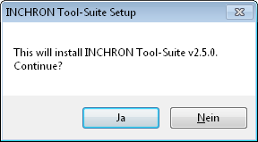
Figure 2.2: INCHRON Tool-Suite Installation Question #

Note:
INCHRON does not guarantee proper operation of the INCHRON Tool-Suite on other operating systems than specified in Section 2.1.2, “Operating System Requirements”.
A welcome window displays recommendations for the installation. Click to continue.
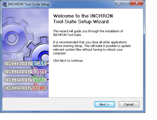
Figure 2.3: INCHRON Tool-Suite Setup Welcome Page #
-
Read the INCHRON Tool-Suite's license agreement carefully. If you agree with the terms and conditions of this license, click .
You cannot install INCHRON Tool-Suite if you do not agree with the terms and conditions of this license.
In this case cancel the installation with .
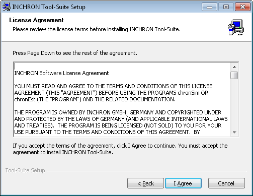
Figure 2.4: INCHRON Tool-Suite Software License Agreement #
-
If you accept the license agreement, setup will ask you which INCHRON Tool-Suite software components should be installed.
The default selection will install all available software components.
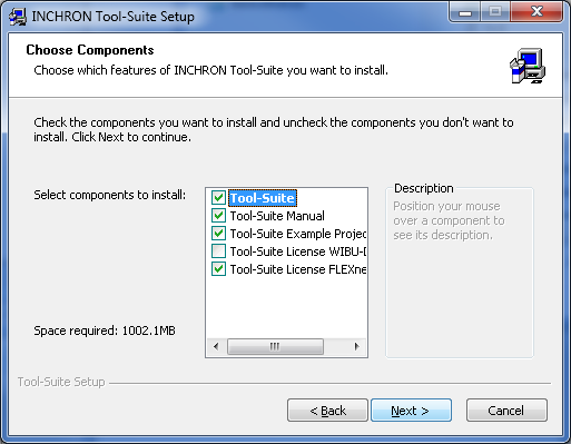
Figure 2.5: Selection of Software Modules for Installation #
Deselect all program modules that you do not need and want to be excluded from installation by ing the respective checkboxes.
Confirm your selection with .
In the next step you will be asked to provide an installation path for your INCHRON Tool-Suite installation. You can manually modify the default installation path by clicking .
A dialog appears for choosing a custom installation directory.
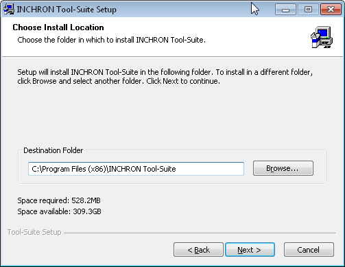
Figure 2.6: INCHRON Tool-Suite Installation Path #
Confirm your selection with .
INCHRON Tool-Suite setup has now collected all relevant information for installing INCHRON Tool-Suite.
Click .
The installation starts. You can observe the progress and all details of the installation on the screen. Please wait until all data is saved onto your hard disk. This may take several minutes.
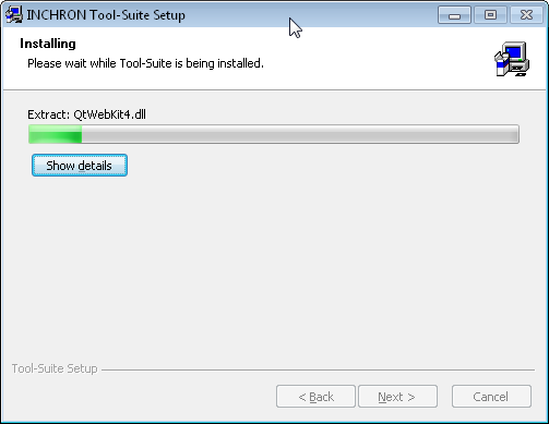
Figure 2.7: Installation Progress #
-
After the installation of INCHRON Tool-Suite you will be asked to confirm the installation of 3rd party tools.
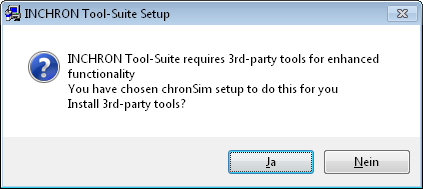
Figure 2.8: Installation of 3rd Party Tools #
-
Confirm with or abort the installation of 3rd party tools by clicking on .
Only the selected software modules will be installed. If you already have appropriate versions of the 3rd party tools installed on your computer, you will be asked if you want to re-install them.
Follow the installation instructions of the respective 3rd party tools installers.
To finish the installation click on .
Figure 2.9: The Installation is Complete #
If you selected the "License WIBU-Dongle" component in Step 8 the computer needs to restarted before using the Tool-Suite.
2.2.2 License Management #
The INCHRON Tool-Suite comprises different tool options namely chronSIM, chronVAL, chronEST, chronBUS, chronVIEW, chronOPT and chronView which may be used separately. The usage of any of these tool options requires a license option. The license may be available either as USB dongle or FLEXlm license. In both cases single-seat as well as network licenses are possible.
The configuration of a license server and the management of licensing options to be used is done with the Manage Licenses dialog from within the INCHRON Tool-Suite. Server license allocation may be limited by restricting any workstation to a single instance of the Tool-Suite application see Section 4.4.1, “General Settings”). Changing the current set of INCHRON Tool-Suite tool license options is done as follows:
Start the INCHRON Tool-Suite with → → → .
In case no simulation or validation license is configured the Manage Licenses dialog will appear. Otherwise
Select → .
The Manage Licenses dialog shows up.
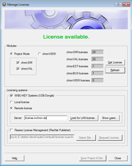
Figure 2.10: Manage Licenses Dialog #
Select the appropriate tool options , , and press .
The License available will be shown if the selected options are covered by your license server or license dongle.
the dialog and restart the INCHRON Tool-Suite.
In case you selected the option chronVIEW only, INCHRON Tool-Suite will directly start in simulation mode instead of project mode.
2.2.3 License Management with WIBUKEY Systems #
2.2.3.1 Separate Installation of Dongle Software #
In case INCHRON Tool-Suite is configured to use the WIBU-KEY Systems license mechanism all license information is stored on an USB dongle. By default the dongle software is installed during the INCHRON Tool-Suite installation. However, you may also install the dongle software separately.
This is done as follows:
Close all other running applications.
Terminate any WIBU-KEY-Server already running e.g. with the context menu of the WIBU icon in the task-bar
Double-click SETUP32.EXE from the
WibuKeyfolder on the INCHRON Installation CD.Follow the instructions on the screen.
The installation program displays the identified operating system and lists all files required for the dongle.
Clicking will copy and install all listed files onto your hard disk.
-
If you encounter an error during the installation, you should restart your computer and start again from a).
After successful installation a new folder
WIBU-KEYcan be found in → .
Note:
To configure INCHRON Tool-Suite for using a WIBU-KEY based license you have to check WIBU-KEY Systems (USB-Dongle) in the Manage Licenses dialog (see Figure 2.12, “Valid WIBU-KEY License”). In case of a local license (local connected USB dongle) also check the Local License option.
INCHRON Tool-Suite automatically checks on every start for the dongle and the dongle software. With a "single license" the dongle is required to be connected to your computer's USB connector when INCHRON Tool-Suite is running. With a floating license the dongle software should be installed onto a separate constantly available computer in your network. In order to use your floating license the dongle must remain in the USB connector of the separate computer. Accessing the floating license may be restricted by a firewall. In such a case, please contact your system administrator.
2.2.3.2 Configuration of a License Server #
In the Manage Licenses dialog you may configure a network license server instead of using a local license dongle. To select a network license server do as follows:
Select → .
The Manage Licenses dialog appears.
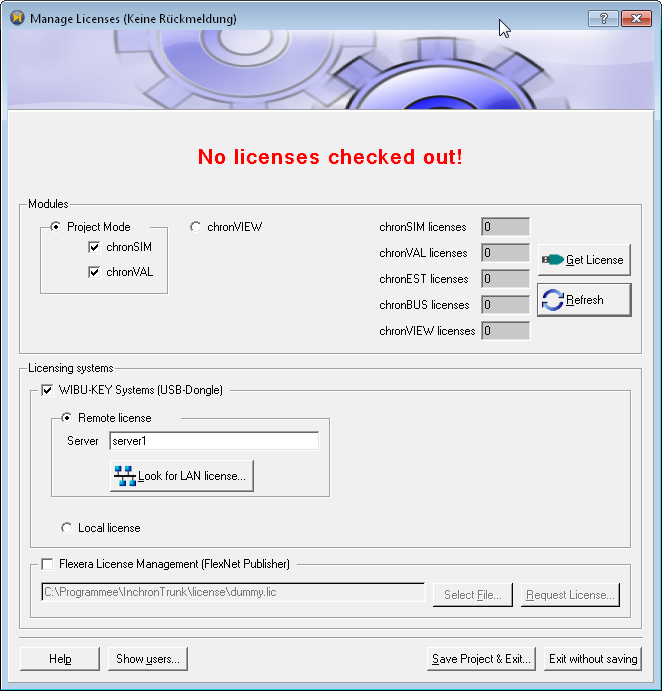
Figure 2.11: Manage Licenses Dialog #
-
Check the Local License checkbox if you have plugged the INCHRON USB license dongle directly into your computer's USB port.
If you have a INCHRON license server in your local area network or on the Internet, enter the server's hostname or its IP address into the Server input field.
Click on .
INCHRON Tool-Suite checks if there is a license dongle connected to your PC or if the license server is available. If successful, the status will change to License available.
Figure 2.12: Valid WIBU-KEY License #
In case searching the license was not successful, check if your license server is running and the network is up and/or the license dongle is plugged in correctly. Then repeat steps 2 and 3
INCHRON Tool-Suite periodically checks for the license dongle or its connection to the license server when running. In case the license check fails, the license manager dialog appears and the Tool-Suite is paused. If the license check failure was only due to a temporary glitch, the dialog will automatically disappear and INCHRON Tool-Suite will continue with normal operation.
In a network license environment the license server must be
constantly available for proper operation of the INCHRON Tool-Suite.
Make sure that legitimate users can access port
22347 (TCP and UDP) on your license server.
We strongly advise you to protect your license server from
unauthorized access by making use of a firewall.
Please find more information on how to run a network license server in the windows start menu under → → → .
2.2.4 License Management with FLEXlm #
Alternatively to using a USB dongle the Flexera FLEXlm® license mechanism may be used. A FLEXlm® license is bound to the host ID of your computer or the network server respectively. The FLEXlm licensing mechanism requires no additional Flexera software to be installed on your computer.
2.2.4.1 Selection of The License Mechanism #
In order to switch to the FLEXlm® licensing mechanism select → from the menu. In the Manage Licenses dialog (s. Figure 2.13, “Manage Licenses Dialog with Activated FLEXlm License”). Check the Flexera License Manager (FlexNet Publisher) option.
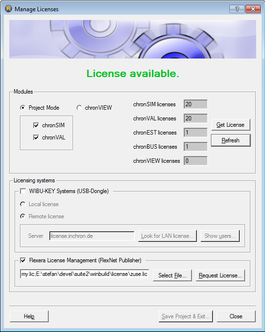
Figure 2.13: Manage Licenses Dialog with Activated FLEXlm License #
2.2.4.2 Installation of The License File #
The FLEXlm® licensing
mechanism requires a LIC
license file in the license
subdirectory of the INCHRON Tool-Suite installation directory. The
license file can be obtained by clicking on Request
License.... It opens a dialog which already contains
your Host ID. You have to add your invoice number and your address.
The buttons Copy to Clipboard or
Create E-Mail both create the content of an
email which you can send to <license@inchron.de>. For
this purpose your configured email tool is started, the Tool-Suite
does not send any emails on its own.
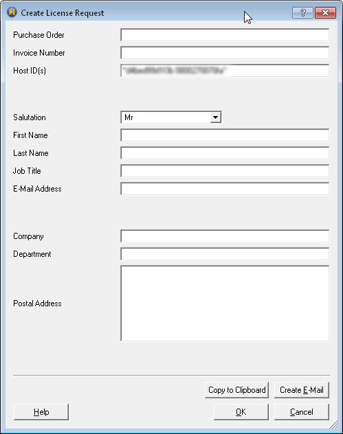
Figure 2.14: Request License Dialog #
Important:
Please take care that in case of a FLEXlm server you have to use the Host ID of the server, not the one of your desktop computer.
Another way to request a license is as follows:
Use the windows start menu to open the command shell.
Change to the folder
licenseof your INCHRON Tool-Suite installation.Invoke the program lmhostid.exe.
The host ID of your computer will be queried and displayed.
Send the Host ID together with the number of your INCHRON Tool-Suite invoice to <license@inchron.de>.
INCHRON will send you a license file which has to be stored in the
licensefolder of your INCHRON Tool-Suite installation.Restart the INCHRON Tool-Suite.
2.2.4.3 Usage of a License Server #
The FLEXlm® license mechanism may also be used with a network or floating license. For this you need a license file on your license server, which has to be copied to each client installation.
First use the lmhostid.exe application to get the server host ID and request a server license file from INCHRON as described in the previous section.
Copy this license file together with the program inchrond.exe to the license server.
On each client copy the same license file to the
licensefolder of your INCHRON Tool-Suite installation.Restart the INCHRON Tool-Suite.
In order to use a network license the license server must be running and connectable by the client.
2.2.5 Selection of Tool Options #
In large installations it is common that a company acquires a different number of licenses for e.g simulation (chronSIM), validation (chronVAL), and trace analysis only (chronVIEW). In such a case it is important that each installation of INCHRON Tool-Suite occupies only the required tool license options.
The selection of required license options can be changed as follows:
Select the menu → .
The Manage Licenses dialog opens (s. Figure 2.12, “Valid WIBU-KEY License”).
In the lower part of the dialog is a set of checkboxes for the tools. Select the licenses you want to use.
The license is requested immediately and the result is displayed.
Close the dialog.
If you change from or to trace analysis (chronVIEW) you have to restart the INCHRON Tool-Suite for the changes to become effective.
When started chronVIEW comes up with the Simulator Window. There you can import trace files immediately. This function is also contained in chronSIM. Thus for comparison of simulation results with measured traces once in a while you do not need to change the license options every time.
2.2.6 Verifying your Installation #
The installation verification is exemplified with an example project.
Start the INCHRON Tool-Suite with → → → .
INCHRON Tool-Suite splash screen will shown and the Tool-Suite starts in project mode.
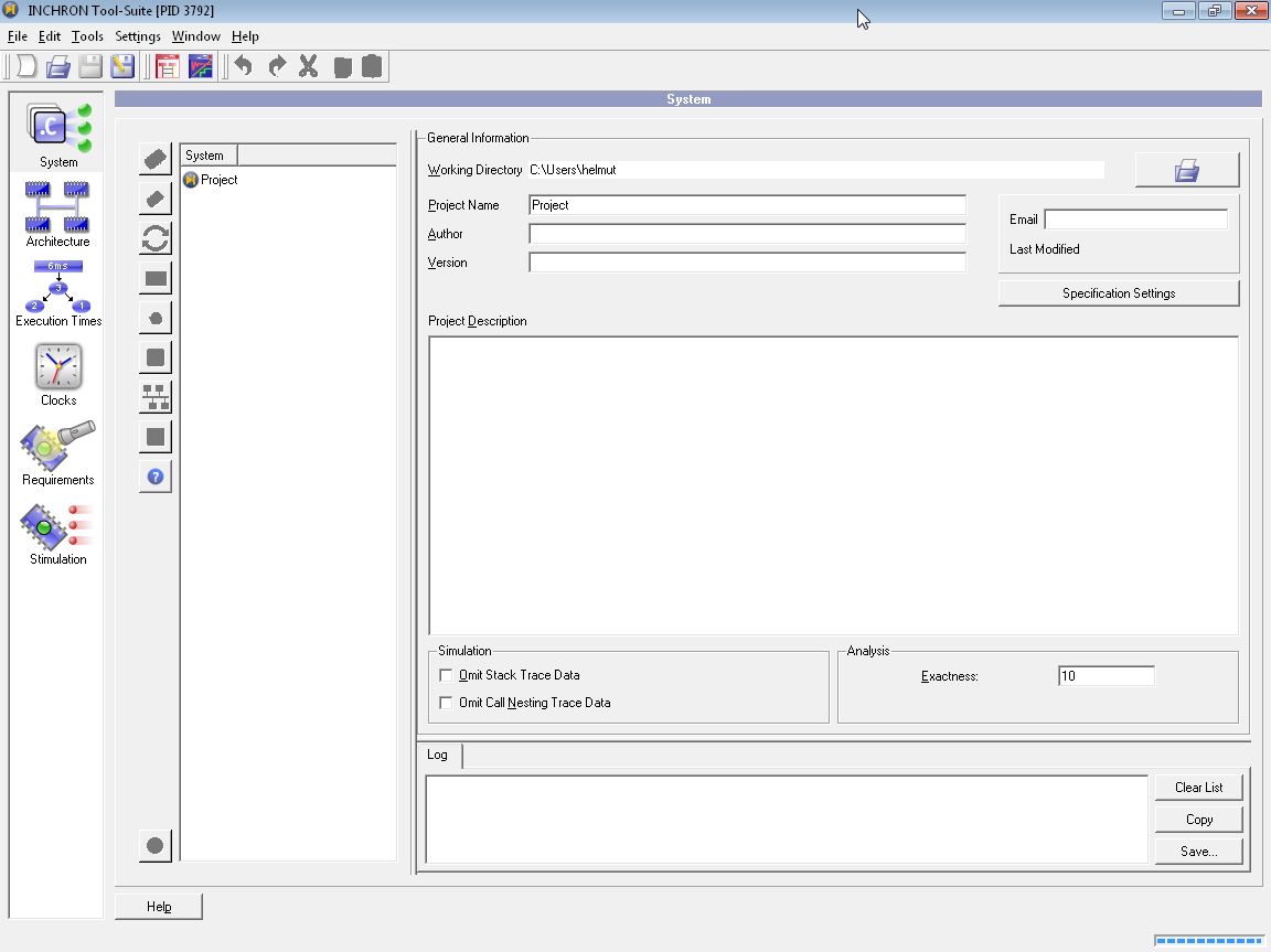
Figure 2.15: INCHRON Tool-Suite Project Window #
From the menu choose → .
The file open dialog for example projects appears.
Open the
dectsubdirectory and select thedect.iprproject file.Confirm with .
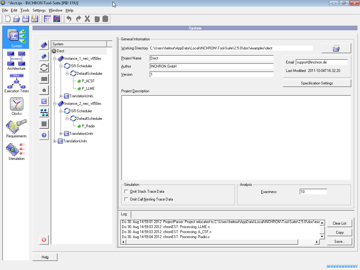
Figure 2.16: INCHRON Tool-Suite Project Window with Example Project #
-
During preparation of the simulation a progress dialog is displayed.
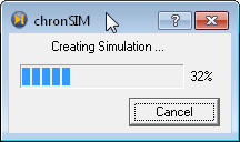
Figure 2.17: Progress Dialog During Simulation Preparation #
After generation of the executable simulation model the INCHRON Tool-Suite Real-Time Simulator window opens.
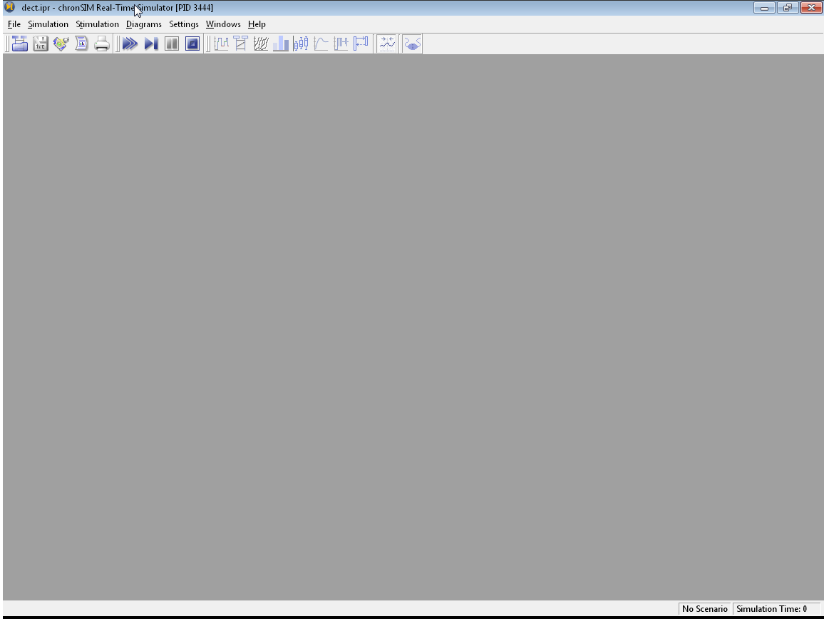
Figure 2.18: INCHRON Tool-Suite Real-Time Simulator Window #
If the generation of the simulation fails you will be notified with an error pop-up window.
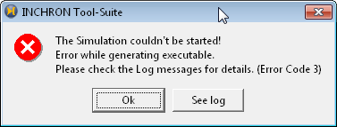
Figure 2.19: Simulation generation failed #
In this case you should uninstall INCHRON Tool-Suite and repeat the installation procedure. If the re-installation does not succeed contact your contractual partner.
-
An (empty) State Diagram window opens.
-
The State Diagram window will show a timeline of processor states as x/t diagram x/t diagram. If necessary adjust the vertical of timescale with the and buttons in the toolbar.
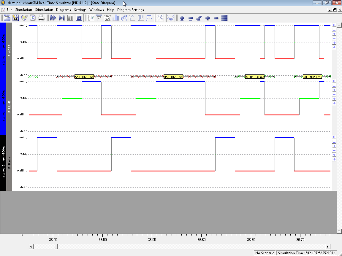
Figure 2.20: State Diagram Window During Simulation #
By successfully simulating an example project the installation of the INCHRON Tool-Suite is verified.
Terminate the simulation with → .
Close the INCHRON Tool-Suite Real-Time Simulator window with → .
Terminate the INCHRON Tool-Suite with → .
2.3 Configuring Python Scripting Support #
Python scripting support for system models comes as an extra software package (which is contained in the regular Tool-Suite installation).
After installing the INCHRON Tool-Suite follow the following procedure to install python support:
-
Download and install the latest release of python 2.7 from the python.org download site" (https://www.python.org/downloads/)
-
Open the
addonsdirectory of the Tool-Suite installation. -
Run the MSI installer called
inchron-model.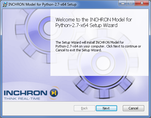
Figure 2.21: Install wizard for the INCHRON Tool-Suite Python Addon #
2.4 Configuring the IBM Rational DOORS Integration #
The INCHRON Tool-Suite has built-in support to connect to an IBM Rational DOORS server and to import and export requirements from and to the DOORS database.
The connection to the DOORS database as well as the attribute mapping must be configured to match the DOORS server configuration. The procedure, the mechanism for deploying a predefined configuration, and the prerequisites for the integration itself are described in the following sections.
2.4.1 Prerequisites #
The connection to the DOORS database is based on Open Services for Lifecycle Collaboration (OSLC). It supports Requirements Management (RM), version 1.
IBM Rational DOORS offers this interface via the DOORS Web Access (DWA). The Tool-Suite requires at least DOORS 9.3.0.4 and DOORS Web Access 1.4.0.4. The following sections assume that these DOORS components have been installed. Additionally administrative permissions on the DOORS database are required for configuration.
2.4.2 Configuration #
The INCHRON Tool-Suite OSLC integration can be configured using a web browser. Select → to start the configuration. On an unconfigured system the Initial Configuration Page will also be shown when selecting any other DOORS-related operation.
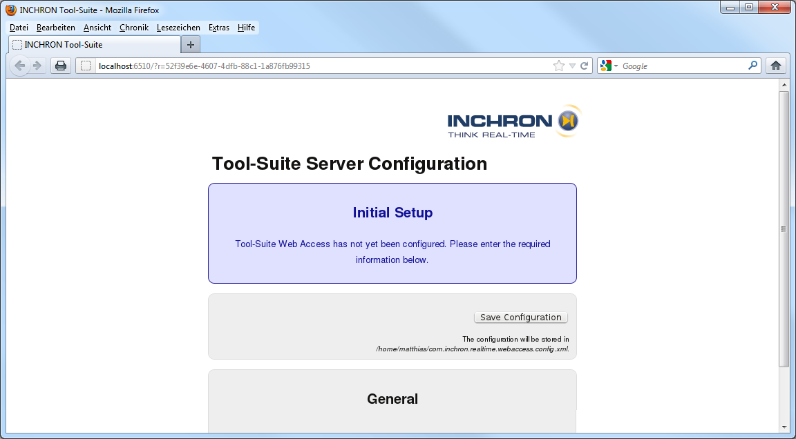
Figure 2.22: The Initial Configuration Page #
At the top and the bottom of the page a Save Configuration button is located. It stores the actual values to an XML encoded file.
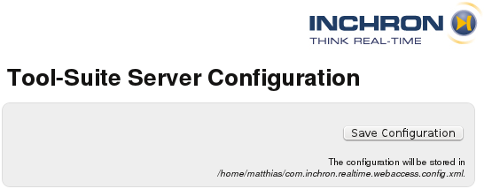
Figure 2.23: The top section of the Configuration Page #
The OSLC based connection to the DOORS database is a two-way
communication. Therefore the Tool-Suite also opens a local TCP port and
listens for connections. In the General section
this port can be configured. The port is only reachable from localhost.
The Log Level can be configured. All messages are shown in the Log Messages Window of the Tool-Suite.
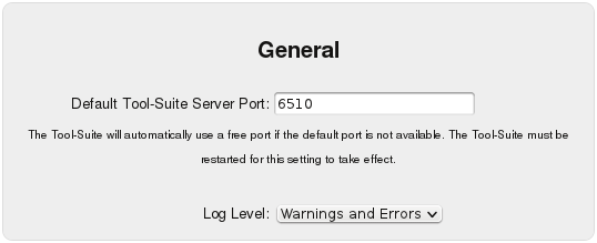
Figure 2.24: The General section of the Configuration Page #
The connection to the DOORS database has to be configured in the DOORS Web Access section. The options are:
-
The Root Services URL identifies the connection point to the DOORS database. Usually it contains the scheme
https://, a hostname, a port and the path component /dwa/public/rootservices. The hostname can be a fully specified hostname, a local hostname, or an IP address. The port number is defined by the configuration of the DOORS database with the default being 8443. Ask your DOORS administrator for the actual values. Valid examples are:https://doors.example.com:8443/dwa/public/rootserviceshttps://localhost:8443/dwa/public/rootserviceshttps://10.10.17.42:8443/dwa/public/rootservices
-
In addition to the user credentials the INCHRON Tool-Suite has to authenticate itself as a registered application for the DOORS database. For this purpose the OAuth Consumer Key and the OAuth Consumer Secret are used. Enter the same values here which you have registered in the DOORS database.
-
The name for an imported requirement is taken from the attribute specified in the Tool-Suite Source Attribute field. The default is
dc:title. -
In the same way the name of the attributes can be specified where the chronSIM and the chronVAL results are written into. These fields have to be added by the DOORS database administrator before they can be used. The same value is allowed for the chronSIM Target Attribute and the chronVAL Target Attribute. If this is the case the results are either overwritten or prepended according to the strategy selected for New Test Results.
-
The dropdown-box New Test Results defines the strategy which is used when results are exported to DOORS and there is already a result from earlier simulations or analyses. You can change between Overwrite (keeps only the last result), Prepend (the last result is the first paragraph) or Ask (which requires user interaction).
-
Ignore SSL Error: Continues the import and/or export process even in the case of errors during the SSL handshake. Otherwise the error is shown and the process is canceled.
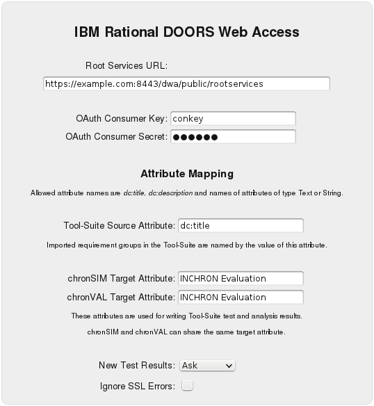
Figure 2.25: The DOORS Web Access section of the Configuration Page #
At the bottom of the configuration page the Save Configuration button is repeated. Hyperlinks provide access to the INCHRON Support and to the INCHRON web site.
Figure 2.26: The bottom section of the Configuration Page #
2.4.3 Deploying a Predefined Configuration #
The configuration of the connection to the DOORS database can be shared by multiple users by performing the following steps:
-
Install the Tool-Suite and start it as an ordinary user.
-
Edit the IBM Rational DOORS Settings (see Section 2.4.2, “Configuration”).
-
Save the configuration settings.
A file
com.inchron.realtime.webaccess.config.xmlis created in the directory%USERPROFILE%. -
Copy the file
com.inchron.realtime.webaccess.config.xmlto the installation directory of the INCHRON Tool-Suite. This is one level aboveSuite.exe.
Now every user running this Tool-Suite installation will use the set configuration.
2.5 Uninstall INCHRON Tool-Suite #
To uninstall INCHRON Tool-Suite follow the instructions below:
-
Exit the INCHRON Tool-Suite.
Save all your simulation results and project files on an external drive. Make sure to preserve the folder structure.
Start the software management panel by clicking → → and select Software.
The list of installed programs appears.
Select INCHRON Tool-Suite from the list.
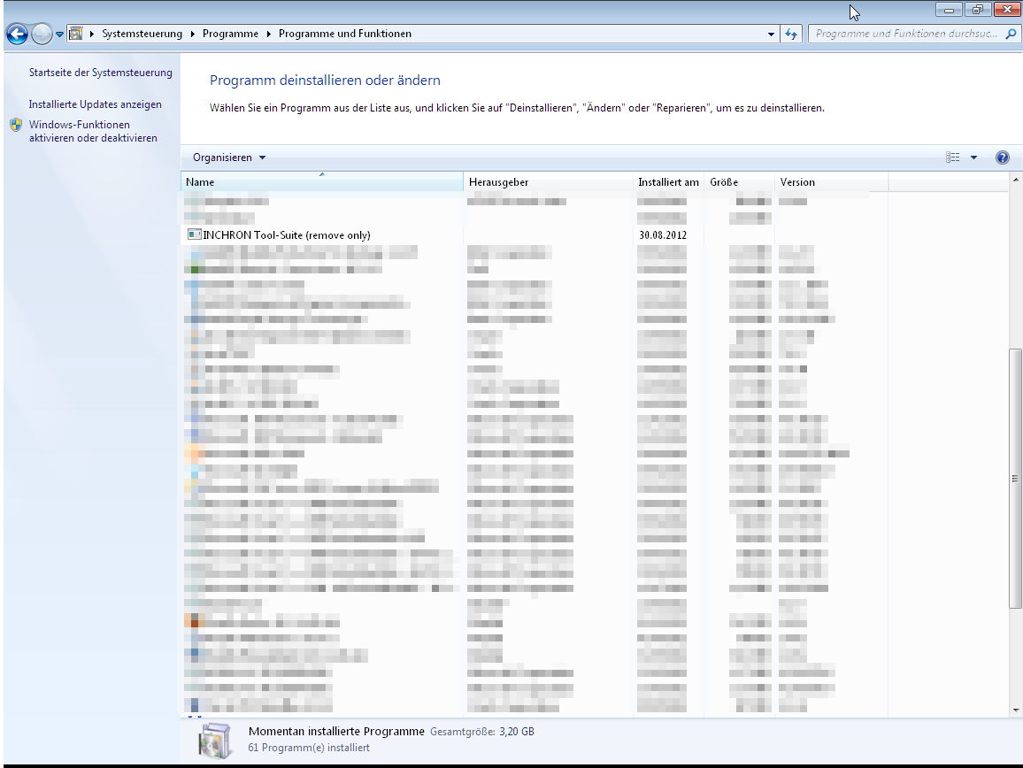
Figure 2.27: Windows Deinstallation Window #
Click on and follow the instructions on the screen.
These programs may be removed separately with → → → → → .
2.6 Re-install INCHRON Tool-Suite #
After deinstallation the INCHRON Tool-Suite may be re-installed with the same procedure as on initial installation.
3 Basics #
The following chapter gives you a brief introduction in the structure and handling of INCHRON Tool-Suite.
3.1 INCHRON Tool-Suite Features #
The term system architecture is always regarded as the view on the target system. An INCHRON model of the target system consists of:
The number and type of microprocessors
The wiring of processors in multiprocessor systems
The (real-time) operating system in use
The mapping of tasks on processors
The mapping of runnables on tasks
The selection of scheduling methods and strategies
The assignment of task and interrupt priorities
The specification of external peripherals like interrupt inputs, parallel ports and communication interfaces.
The modeling of external stimulation.
All these aspects of an embedded system are edited with the graphical model editor of the INCHRON Tool-Suite. Interoperability with external models is provided with OSEK OIL, DBC, FIBEX and AUTOSAR import features. The creation and manipulation of system models may also be scripted using the inchron python modeling API.
The optional component chronSIM connects the functional simulation of the source code of your embedded system with the analysis of execution times of the real target system by chronEST. The optional component chronVAL allows the analysis of real-time capabilities. To achieve this, the user has to specify various aspects of the target system using the modules of the INCHRON Tool-Suite GUI.
The module system shows a unified view of the system models hardware and software. Microprocessors are defined to be mapped to processes or tasks and source files.
Based on this information and with aid of the optional chronEST component the INCHRON Tool-Suite will estimate static execution times of functions and processes. Estimated execution times may be overridden individually by the user
The purpose of module architecture is to define the hardware mappings between microprocessors and communication controllers and buses. Thereby the communication relations between microprocessors are defined
In a multiprocessor system each processor has its own view of time, a clock triggered by its quartz. A major feature of the INCHRON Tool-Suite is that the simulation with chronSIM takes into account all effects of deviating local times due to different drifting microprocessor clocks. For that purpose parameters like granularity and the drift or range of values are specified for each clock individually.
The objective of chronSIM simulation and chronVAL validation with the INCHRON Tool-Suite is to asses whether a given system meets specific requirements under different scenarios of external stimulation. If this is not the case INCHRON Tool-Suite allows to analyze the causes for requirement violations and provides a means to evaluate system model variants without the need of prototypes in real hardware.
Real-time requirements like response times and functional requirements like stack limits are defined within INCHRON Tool-Suite and requirement violations are indicated in the simulation diagrams.
A chronSIM simulation can be stimulated in flexible ways with different stimulation scenarios. The module stimulation of the Tool-Suite allows for configuration of stimulation scenarios ranging from simple periodic signals to complex scenarios with mutual dependencies and stochastic generators or even with recorded data from field tests.
For chronSIM simulation the definitions and configurations of the system model are compiled into an independent simulation executable. The resulting simulation model is executed under the control of a timed event-driven simulator. All simulation times recorded and displayed in the various diagrams show real execution times of the target system and have no relation to any execution times on the simulation host.
Due to the compiled simulation the simulation runs much faster than e.g. the interpretation of each instruction of the binary code.
3.2 INCHRON Tool-Suite Modes of Operation #
INCHRON Tool-Suite uses three different modes of operation and an additional viewer only mode:
Project Mode
The project mode is in fact the INCHRON project editor which allows to define all aspects of the system model used by the INCHRON Tool-Suite components chronEST, chronSIM, chronBUS and chronVAL
Simulation Mode
The simulation mode simulates and analyzes the target system based on the project settings and its configuration.
Validation Mode
Provides chronVAL validation of the target system by means of chronVAL.
Viewer-Only Mode
A restricted (chronVIEW) license which allows for viewing and analysis of existing simulation traces with diagrams and histograms of the simulation mode.
Each of the first three INCHRON Tool-Suite modes uses a separate application main window. The viewer-only mode uses the same window as the simulation mode. For a better understanding of the following descriptions you may want to start the INCHRON Tool-Suite. After starting the application with → → → the INCHRON Tool-Suite project mode window will appear.
3.2.1 The Project Mode #
In project mode the INCHRON Tool-Suite window is presented as main window for user interaction. It presents different views for editing different aspects of a system model. A detailed description of features of the project mode is subject to Chapter 6, System Modeling.
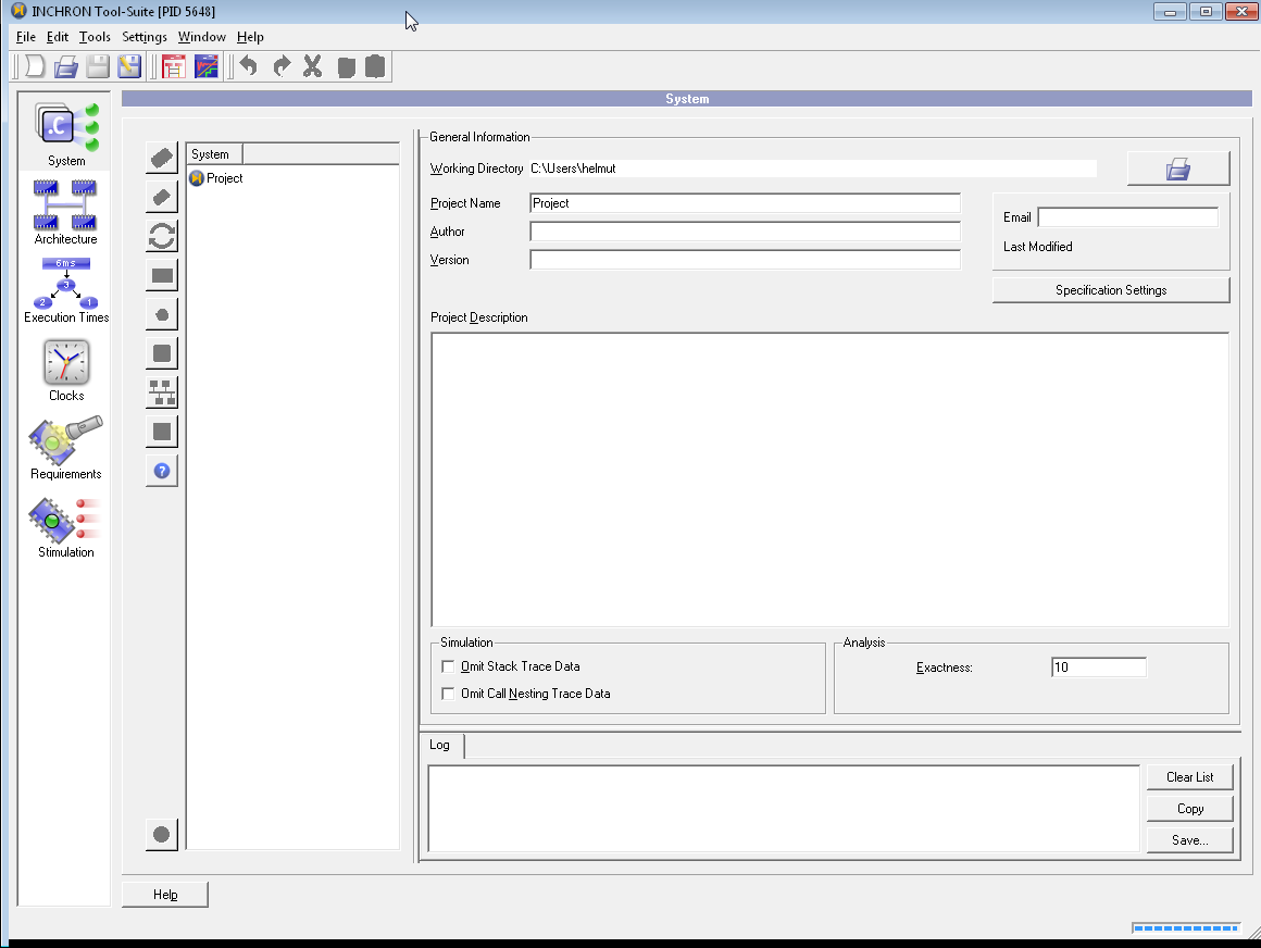
Figure 3.1: The INCHRON Tool-Suite project mode window #
3.2.1.1 The Project Mode Modules #
The editing of a system model is divided into separate modules. Each module is represented by its own icon. All module icons are vertically arranged on the left side of the project mode window. Each module can be activated by ing module's respective icon which will show the modules input masks.
3.2.1.2 Module System: Overall Model View #

This module shows the system models hardware and software components a system tree and allows adding, removing and editing of the components.
See Section 6.2, “Module System” for a detailed description.
3.2.1.3 Module Architecture: Hardware Components and Connection Matrix #

Shows a hardware view of the system tree. Allows for editing of the system's microprocessor and hardware communication interfaces their peripheral components and the connections of peripheral ports.
See Section 6.3, “Module Architecture” for a detailed description.
3.2.1.4 Module Execution Times: Estimated Processor Cycles #

Contains function and process execution times estimated with chronEST.
See Section 6.4, “Module Execution Time” for a detailed description.
3.2.1.5 Module Clocks: Processor Clocks #

This module comprises parameters of system clocks which define the individual time bases of the systems microprocessors and schedule tables of AUTOSAR systems.
See Section 6.5, “Module Clocks” for a detailed description.
3.2.1.6 Module Requirements: Conformance Criteria #

Definition of functional and real-time requirements for the specification conformance of the system. Real-time requirements are expressed as time budgets of e.g. processes, functions or processing steps. Criteria for functional requirements are e.g. function stack usage.
See Section 6.6, “Module Requirements” for a detailed description.
3.2.1.7 Module Stimulation #

Scenarios for external events and interrupts acting as input on the simulated system.
See Section 6.7, “Module Stimulation” for a detailed description.
3.2.2 The Simulation Mode #
The simulation mode requires the chronSIM license option and is entered by loading and compiling a simulation project from the project mode window. A detailed description of features of the simulation mode is subject to Chapter 7, Simulation. For a better understanding please open the example project from the INCHRON distribution:
Figure 3.2: chronSIM Real-Time Simulator window #
Together with the Real-Time Simulator window the Simulation Control window appears.
The purpose of the Simulation Control window is to enable of disable specific breakpoints. It may be toggled with → .
3.2.2.1 Functions for Simulation Control #
The basic functions for starting and stopping the simulation are available in the menu of the Real-Time Simulator window or with the buttons of the simulation control toolbar. Additional breakpoint functionality is provided by the Simulation Control Window .
Run Simulation.
 The current simulation will be executed.
Step into Simulation.
 The simulation executes a single basic block.
Break into Simulation.
 A running simulation will be stopped (paused).
3.2.2.2 Functions on Simulation Trace Files #
Open Trace File.
 Allows for opening of saved INCHRON simulation traces.
Save Trace File as.
 A Simulation trace will be saved as
 ISF file.
3.2.2.3 Functions for Simulation Visualization #
chronSIM provides a set of diagrams for the visualization of the dynamic system behavior, each offering a view on different aspects of the simulated system. All diagrams can be viewed from the Real-Time Simulator window, which becomes available when starting a simulation or loading a previously saved simulation trace file. The diagrams are available in the Diagrams menu or with the toolbuttons of the diagrams toolbar. Additional diagram functionality for printing or exporting data can be accessed via the windows menu bar or the diagrams context menu. For a detailed description of simulation diagrams see Section 7.7, “Visualization”.
Show Sequence Diagram.
 This diagram shows communication activity between tasks
as well as between tasks and ISRs.
This diagram shows communication activity between tasks
as well as between tasks and ISRs.
Show Stack Diagram.
 This diagram shows the stack usage of tasks over time.
Show State Diagram.
 This diagram visualizes each task's operating system states
running, ready, waiting or dead over time.
This diagram visualizes each task's operating system states
running, ready, waiting or dead over time.
Show Nesting Diagram.
 This diagram shows the nesting depth of functions of a process over time.
Show Load Diagram.
 Shows utilization of microprocessor resources over time.
Create Histogram.
 Show a diagram for the statistical distribution of the time interval
of two events (e.g. process start and termination).
Unlike for other diagram types multiple histogram windows may be open at the same time.
The following images show diagram examples.
Show a diagram for the statistical distribution of the time interval
of two events (e.g. process start and termination).
Unlike for other diagram types multiple histogram windows may be open at the same time.
The following images show diagram examples.
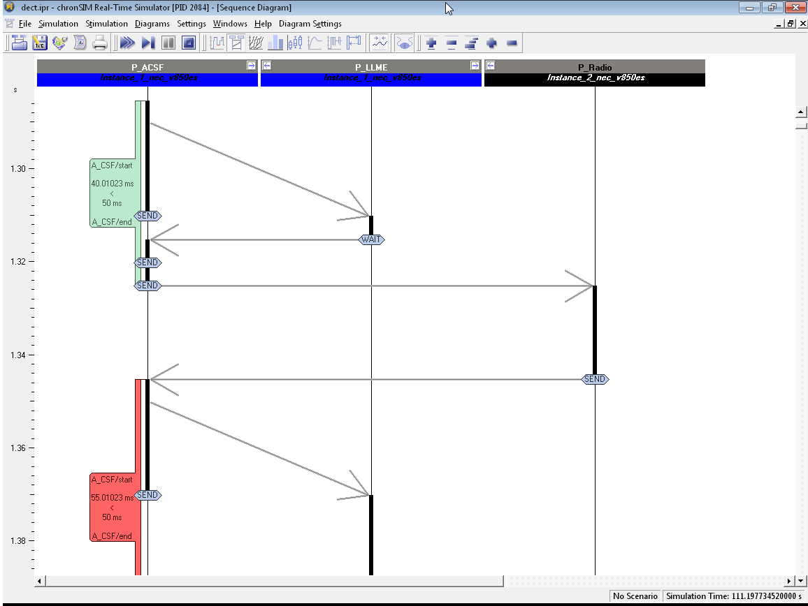
Figure 3.3: Sequence Diagram With Three Processes #

Figure 3.4: State Diagram With Three Processes #
3.2.2.4 Usage of the Simulation Control Window #
The Simulation Control window allows the user to define simulation breakpoints. The following breakpoint conditions are possible:
Time based breakpoints (absolute ore relative)
Event based breakpoints (function, process or user defined events)
Break on RTOS violations
Break on violations of defined limits for recursion, function nesting depth as well as stack size.
That way, the compliance with design requirements may be verified immediately during simulation.
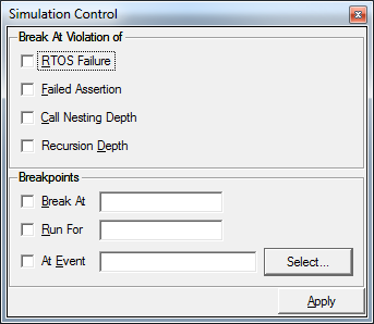
Figure 3.5: Simulation Control Window #
3.2.3 Interactive Modeling with chronSYNTH #
The chronSYNTH mode provides interactive modeling features for simulation diagrams. This facilitates model changes from within the simulatior window, which trigger a simulation and an immediate update of simulation diagrams for an immediate update on any effects of model changes. For that purpose, the context menus of simulation diagrams have a sub-menu offering several actions for model modifications. See Chapter 10, Interactive Design of Dynamic Architectures for details. Any changes can be applied by clicking the Run Simulation toolbutton in the Project Window which will restart of the simulation. Once finished the diagrams in the Simulator window will be updated accordingly.
Important:
The immediate update is only possible for models without source code.
3.2.4 The Validation Mode #
The validation mode requires the chronVAL licensing option and is entered from the project mode window. A detailed description of features of the validation mode is subject to Chapter 8, Validation. For demonstration open the validation example project:
Open the dialog for example project with → and select the project
distributed.iprfrom thechronVAL/distributedfolder.-
 Enter validation mode with
→
or alternatively with the shown icon from the toolbar.
Enter validation mode with
→
or alternatively with the shown icon from the toolbar.The chronVAL Response Time Composition and chronVAL Event Spectrum Viewer windows open.
Wait until chronVAL analysis of the project has finished. While not finished the Event Spectrum Viewer will display an Analyzing... message.
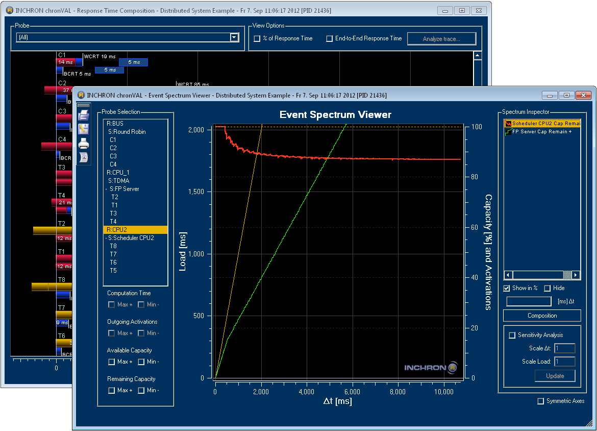
Figure 3.6: The chronVAL Validation windows #
3.2.5 The Viewer Mode #
The chronVIEW license option is a restricted mode for using the functionality of INCHRON Tool-Suite simulation diagrams on simulation traces. This includes viewing saved chronSIM traces and the import of custom CSV traces.
In chronVIEW mode INCHRON Tool-Suite will start with a simulation viewer window. The configuration of a chronVIEW license option is described in Section 2.2.2, “License Management”.
The usage of the diagram functions is like described in Section 7.2, “Running a Simulation”.
Opening a simulation trace is done as described in Section 7.8.2, “Loading a Trace-File”.
The import of custom trace files includes the automatic creation of a basic system model which may be opened in the model editor via (chronSIM license option assumed). Management of real-time requirements for imported traces is also available after opening the model editor.
4 Projects #
An inchron project comprises an embedded system's hardware and software model together with additional meta information, specification of real-time behaviour and requirements, generic tool settings and specific settings and configuration for reporting, chronSIM, chronVAL and chronOPT.
An INCHRON project is saved as an IPR file in an XML representation.
This project file contains all task specifications, all source modules including their parameters,
as well as paths to their files.
The Tool-Suite system model editor therefore requires the user to specify a project folder at runtime. By default, the project folder is created in the user's personal folder. With the default setting, the Tool-Suite expects to find all model specifications and associated files in this folder.
If an alternate folder is specified, it will apply to your project file, the project's C source code modules and will be the default search location for any additional model descriptions (e.g. OIL, DBC and FIBEX files).
Name and file identifiers used in simulation models are case-sensitive.
Files with the IPR file name extensions
are associated with the Tool-Suite application
so that ing
will automatically start the Tool-Suite and load the project.
Important:
The project name has to be conform with your host's operating system conventions. INCHRON recommends the letters A to Z, a to z, the numbers 0 to 9 and the special characters dash and underscore as allowed characters for file names and identifiers. All other characters might cause problems related to the interoperability with other programs like backup programs.
4.1 Project Creation #
After being started the INCHRON Tool-Suite starts up with an empty project.
-
Select the Module System
and there select the project item in the system tree
The project's global properties and settings are displayed on the right hand side as shown in the screenshot below.
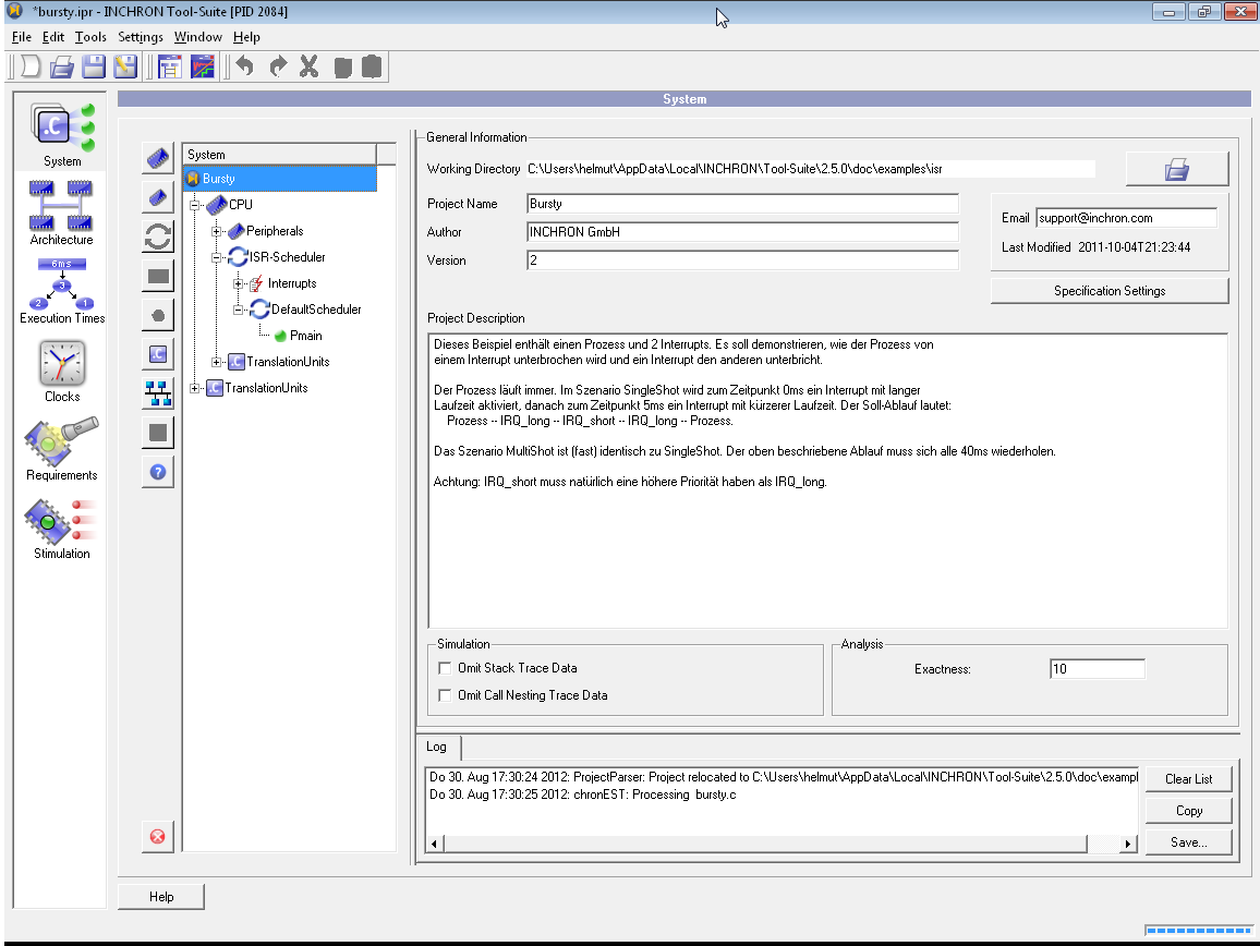
Figure 4.1: Example of Project General Settings #
The project property view contains the following informational items on global project settings:
 Project Directory
The location of your project's working directory on your file system. By default the project directory is set to the personal folder the user. Since the project related files are stored in the project's working directory it is recommended to use a separate folder for each project. In order to select a working directory the button with the shown icon.
Project name
Enter a unique project name. The project name will be used as basename for the project file.
Author and Email
Version and Last Modified
While the Last Modified field gets updated whenever the project is loaded or saved the Version has to be edited manually.
Project Description
This input is intended for a textual description of your project. You can modify and add information at any time, thus recording your project's progress.
Group Analysis
The Exactness parameter is the number of iterations after which the chronVAL analysis switches to approximation. A higher value for exactness will decrease the pessimism of calculated worst case response times, with the cost of increased analysis computation time.
Group Simulation
If Omit Stack Diagram is checked chronSIM simulation will not record any function stack changes.
if Omit Call Nesting Diagram is checked the chronSIM simulation will additionally suppress the recording of function entry and exit events (including AUTOSAR Runnables).
if Omit Implicit Event Chains is checked the simulation will not record information for tracing the connections of implicit process activation chains and dataflow chains
-
if Global Simulation Replacement override Chains Use this option to globally override the Simulation Replacement of processes and runnables. This does only apply to those processes and runnables with active Simulation Replacement, i.e. not to processes and replacement with assigned entry function.

Tip:
Each of the "Omit" options above can be used to reduce the size of simulation traces. This comes with the tradeoff of reduced functionality of diagrams, requirement evaluation and reporting for omitted elements.
Log
Log messages from e.g. loading projects, parsing source files and generating simulation
You may save your project settings using
→
or by clicking the
 button from the toolbar.
The file extension
button from the toolbar.
The file extension IPR will be appended automatically.
4.2 Modifying the Project Directory #
In some cases you may wish to reorganize your projects on your hard disk, including INCHRON project files and their associated files.
You may use your operating system's tools to move and reorganize your projects in your file system.
The project file of a model contains information about the associated files, including their paths. Files in the project directory or a subfolder will be stored with relative paths. We recommend to also save the project file in the project directory or a subfolder thereof.
After the reorganization of the files associated to your project, the internal integrity of your project files is temporarily inconsistent.
When a project file is loaded into the Tool-Suite after moving in the filesystem, the project's internal file path and file references will be adjusted automatically. The project status will be set to modified and thus has to be saved with Ctrl–S to get a consistent project file.
4.3 Load and Save Projects #
If any of the project's specifications are modified the simulation project file should be saved.
For saving a project use
→ (Ctrl–S)
or click the  icon from the toolbar.
Alternatively to write to a new project file
in order not to overwrite an existing project file use
→
or click the
icon from the toolbar.
It is also possible to checkout a project from a subversion repository or to put a project under version control, see Section 12.3, “Version Control for Projects”.
4.4 Global Settings #
In addition to the project directories of your projects and their associated files, some paths to 3rd party tools required for enhanced functionality may be customized.
These additional 3rd party software tools were installed to your computer during the installation of INCHRON Tool-Suite and are used for the output of visualizations of chronSIM's simulation results.
Beside the paths to the additional software tools the length of the recent project list can be adjusted.
The configuration of an editor for source files is not required. chronSIM will use the default application which is associated with the file type.
The Tool Settings dialog is available with → . The dialog contains the two tabs General for general settings and Updates for automatically checking for Tool-Suite updates.
4.4.1 General Settings #
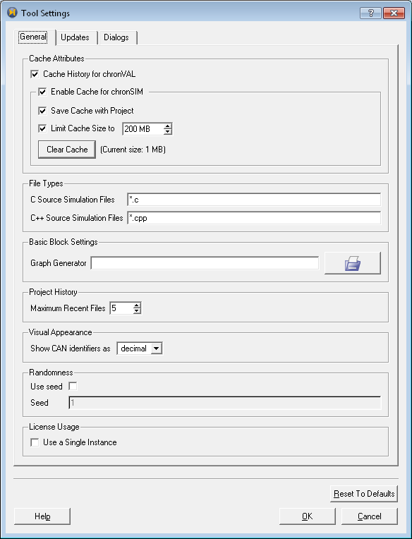
Figure 4.2: General Settings Dialog #
4.4.1.1 Caching of Intermediate Files #
In order to speedup source code parsing and the generation of a simulation model the INCHRON Tool-Suite may use a cache of intermediate results on your hard drive.
Objects in the cache are used in favor of re-compilation if the cache object is more recent than the timestamp of the corresponding C source file and included header files. Also, cache data is always specific to a INCHRON Tool-Suite release so that cache data generated with one Tool-Suite release will not be used when running a different release.
The cache behavior may be influenced as follows:
Enable Cache is a global switch to enable the cache. If deactivated its contents will not be deleted automatically.
If option Save Cache with Project is checked, the location of the cache will be in the project working directory (see Section 4.1, “Project Creation”). Otherwise it will be located in the central user directory.
If Cache History for chronVAL is checked the calculation of chronVAL response times will be cached. This speeds up subsequent process state diagram calculation with the tradeoff of increased memory footprint during analysis.
With the currently selected cache location will be cleared. This is useful to cleanup disk space from cache data no longer used.
4.4.1.2 Source Code File Extensions #
Generally the Tool-Suite treats only files of the type .c
as C source code and .cpp as C++ source code.
By changing the field File Types you can adapt
the Tool-Suite to accept other file types in your projects.
Enter the file types as *.c as shown in Figure 4.2, “General Settings Dialog” . Multiple file types have to be separated by a semicolon (;).
The file types entered here can also be used as filters in the file dialogs when adding files to your project. They are stored permanently, too.
4.4.1.3 Basic Block Graph Viewer #
In order to view graphs resulting from the basic block analysis of the model's source code the external program dot.exe from the ATT GraphViz package is used. The directory path of the program is usually configured during Tool-Suite installation and does not need to be changed.
4.4.1.4 Project History Length #
Maximum Recent Files set the max. number of entries of the → menu.
4.4.1.5 Format of CAN Identifiers #
Packages of CAN messages have a numeric ID which is shown by some components of the INCHRON Tool-Suite. With Show CAN Identifiers as the base of numerical presentation may be changed for your convenience.
4.4.1.6 Initialization of Random Number Generators #
During simulation pseudo random numbers are applied in two cases:
Stimuli generators may be subject to random variation, and
the functions of the task model may explicitly call random generators.
In general random generators of stimuli generators are initialized with a pseudo random seed which results in a new pseudo random stimulation sequence for each simulation run. By checking Use seed random stimulation sequence will be reproducible with a given Seed value (see Figure 4.2, “General Settings Dialog”). The Seed value will be interpreted as a 64bit integer with each bit being evaluated to initialize the random number generator.
Note:
The random generators used by functions called from the Task Model use a constant initialization independent from the seed set. Thus a random stimulation exported from a simulation trace for reuse reproduces only stimulation, but not the sequence of random numbers of random functions used in the Task Model.
An activated seed also applies to the random generators and functions called in the model source code.
Note:
Since these settings are stored globally (project independent) they will also apply after restart of the Tool-Suite and on the batch simulation. However batch simulation provides a command line parameter to override the default seed, (see Section B.2, “Batch.exe”).
4.4.2 Update Settings #
4.4.2.1 Automatic Update Checking #
INCHRON Tool-Suite may check automatically for release updates. This check may also be done manually from the menu.
For configuration of the automatic update check select the Updates tab of the Tool Settings dialog.
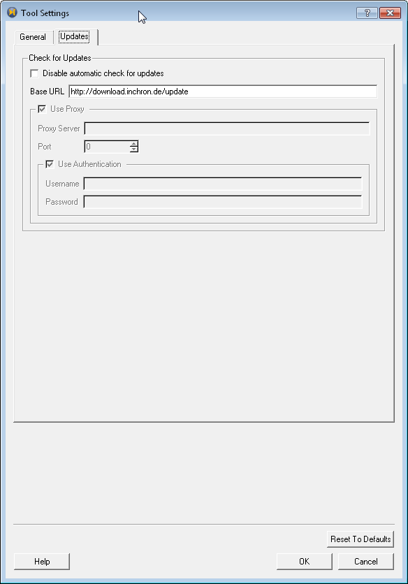
Figure 4.3: Tool-Suite Update Settings #
For checking available updates the INCHRON Tool-Suite will send its release number, build date and the number of the support contract to the INCHRON update server. In case an update is available the information of the update server's response will be shown in the Update Status dialog. It contains the number of the latest available release and the latest build date of the release currently in use.
Note:
An update will not be triggered automatically. Instead it requires a manual download of an installer from the INCHRON download site.
Automatic update checking may be suppressed by checking Disable automatic check for updates.
The Base URL option allows to set an intranet server instead of the INCHRON update server in order to restrict update to releases approved by your responsible department. Please contact your sales partner for details.
A manual update check is triggered with → which will show the Update Status dialog shown below.
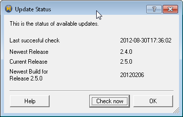
Figure 4.4: Tool-Suite Update Status #
ing Check Now will trigger an update check which will provide the following information items:
Last successful check shows the time of the last successful update check.
Newest Release is the release number of the latest available INCHRON Tool-Suite release.
Current Release is the release number of the currently running INCHRON Tool-Suite.
Newest Build for Release... is the date of the latest build of the currently running release. New builds usually contain bugfixes and minor improvements.
4.5 OSEK OIL Import #
OSEK/VDX is a common standard for real-time systems widely spread throughout the automotive industry.
OSEK/VDX covers the API and behavior of the real-time kernel (OSEK OS) as well as a description language for operating system aspects (OSEK Implementation Language, OIL). Apart from task names and interrupt service routines, the OIL specification file defines task priorities, scheduling methods, synchronization objects like events and resources as well as other attributes.
INCHRON Tool-Suite provides support for importing OSEK system properties from an OIL specification file, which allows you to quickly set up a simulation project, without being forced to manually specify the system's attributes again in the Tool-Suite. This procedure is exemplified in the following sub-paragraph. Additionally you can import attributes from an OIL file into your project any time you want (see Section 4.5.4, “Importing OIL on Existing Projects”).
4.5.1 Create Project from OIL #
You will find the example used in this chapter in the doc\examples\OIL subdirectory of your Tool-Suite installation.
The following example will create a project file in the same directory as the OIL file. If you prefer to leave your installation directories untouched, or if you don't have write permissions in this directory, copy the entire OIL subdirectory to a temporary working directory.
Tip:
As part of the following instructions an INCHRON project will be created in the folder of the OIL file. Thus you may start with copying the OIL file to another destination.
Start the INCHRON Tool-Suite, and select → → from the menu.
The following dialog will be shown.
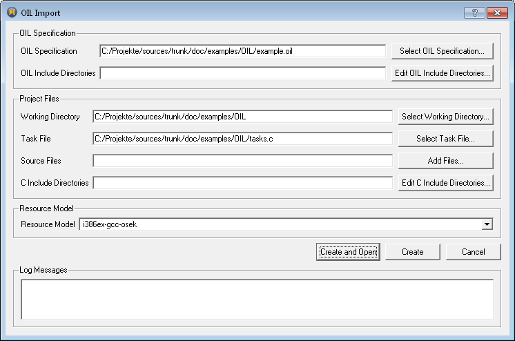
Figure 4.5: OIL Import dialog #
Click on . and select the
example.oilfrom the example directory.Specify any required search paths for the OIL file's
#includedirectives by clicking on the button.Specify the project's working directory by pressing and selecting the example project directory.
-
Add the
tasks.csource file to your project by clicking and selecting this file from the example directory. -
This example does not require any additional C source code files. Hence Source Files the input field should remain empty.
A list of include directories for the C source code can be specified with a dialog available via the button.
-
Use dialog to define the resource type to be used for this project. Select the i386ex-gcc-osek model for this example.
Finish the generation of the project by clicking the button.
INCHRON Tool-Suite reads the specified OIL file and generates an INCHRON project file. The project file will be opened after its generation.
4.5.2 Import Strategy #
For the generation of a project file from an OIL file you must at least provide the system's attributes mentioned above. The attributes comprise the OIL file itself, a working directory, a file containing the implementation of all tasks and a resource type model.
INCHRON Tool-Suite's OIL file analysis provides the name of the system's processor. This name is automatically assigned to the resource instance specified in the resource dialog. Only a processor model with OSEK support can be used. Beyond that, the OIL file contains names and attributes of all tasks which are automatically mapped to the resource instance.
The same applies to interrupt service routines defined in the OIL specification file. An interrupt input peripheral component is created for each ISR detected in the OIL file, which will be connected to the ISR automatically. This allows you to instantly start defining stimulation scenarios on the inputs.
All tasks and ISRs must be defined in the task source file, which in turn has to be specified via the input.
Additional C source code files can be specified using the file browser. These files are added to the project and typically contain function and variable declarations and definitions which are employed by the tasks and ISRs. The definition of tasks in added files is not possible. Tasks and ISR definitions have to comply with OSEK notation.
Close the dialog by choosing one of the following three options:
generates an INCHRON project file, which is saved to the same location and name as the OIL file, but with a .ipr file extension,
generates a project file from the OIL specification and opens the file in the Tool-Suite. In case you already have opened a project, you will be asked to save your modifications and the previous project will be closed.
will abort the generation of the project,
4.5.3 Using Imported Projects #
Any project that was generated from an OSEK OIL file can subsequently be used like any other INCHRON project. For example, you can specify additional microcontrollers or add more source code files.
4.5.3.1 Changing OIL Attributes #
You can modify all settings of the generated project file like any other INCHRON project. This allows you to easily test altered task priorities or a different mapping.
Modified settings cannot be written back to the original OIL file automatically. You will have to manually transfer your modifications back to the OIL file, preferably with the tools provided by your OSEK supplier.
4.5.3.2 Simulation #
Projects generated from an OIL file may be instantly simulated. The activation of tasks at system start follows the specifications from the OIL file.
The INCHRON project file generator adds an interrupt input to the system for each ISR definition found in the OIL file. That way the simulation of stimulation scenarios only requires a specification of a scenario to be added. This allows you to instantly define system stimulations within the Tool-Suite, and thus examine your system in various application environments.
4.5.3.3 Saving Projects #
Any modifications in the project are not transferred to the OIL specification file. Modifications are saved to the INCHRON project file and remain preserved for later simulations.
4.5.4 Importing OIL on Existing Projects #
Alternatively to the creation of a new project based on an OIL file it is alternatively possible to update an existing CPU resource from an OIL description.
Create a project as usually and add the source file to the project.
During the analysis of the OIL description, the Tool-Suite recognizes defined OSEK tasks and ISRS by their keywords. For each task or ISR an entry is added to the system model
Select → → from the menu.
A dialog requests the selection of an OIL file.
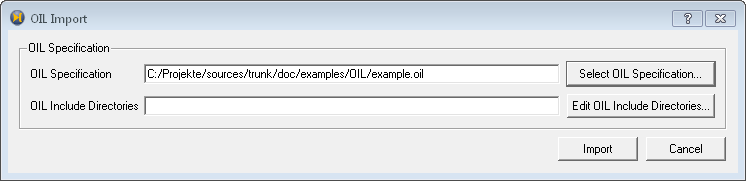
Figure 4.6: OIL File Selection Dialog. #
Select an OIL file and confirm with .
The Tool-Suite reads the OIL file. For each task already contained in the project the attributes from the OIL file are adopted.
Save your project.
There is no connection between your project and the OIL file. Changes done in each of them are not adopted to the other.
4.6 AUTOSAR Import #
As with an OIL file an AUTOSAR ECU Configuration can be imported into the INCHRON Tool-Suite. From the data extracted a project is created.
The AUTOSAR import is as follows:
-
Select → from the menu.
A dialog requests the selection of an OIL file.
-
Select an AUTOSAR XML file and confirm with .
The Tool-Suite reads the file. A new project is created according to the data contained in the project.
-
Save your project.
There is no connection between your project and the AUTOSAR XML file. Changes done in each of them are not adopted to the other.
For further validation or simulation the project has to be extended by either execution times for each task and interrupt service routine, or by a functional implementation in source files. This is done as with any other project.
5 Online Help #
The INCHRON Tool-Suite manual is available as either PDF or via the Tool-Suite's online help system. Using the online help system you may access information on INCHRON Tool-Suite's modules, commands and features at any time from within INCHRON Tool-Suite, using the applications menu.
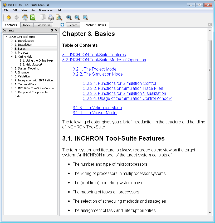
Figure 5.1: INCHRON Tool-Suite Help Window #
5.1 Using the Online Help #
The online help system of the INCHRON Tool-Suite is a full-featured help browser, which allows you to access help information in three ways:
You may select a chapter or section from the table of contents shown on the left,
You may browse the manual index by selecting the tab, or
You may do a full text search by selecting the tab on the right
5.2 Help Support #
In some cases you may need additional assistance to your work on a concrete simulation project. The → item from the menu will show a dialog with support contact information.
6 System Modeling #
6.1 Modules #
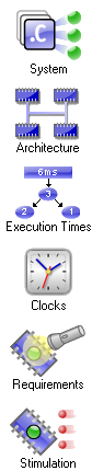
In project mode the INCHRON Tool-Suite window is subdivided into specific modules. These modules represent different views covering different aspects of the creation of a system model:
System
Architecture
Execution Times
Clocks
Requirements
Stimulation
Each Module is selected using the corresponding icon of the module selection bar on the left. The corresponding input masks can be used to specify your system model for chronVAL validation or chronSIM simulation respectively.
You can access the input masks of each module as follows:
Start the INCHRON Tool-Suite by selecting → → →
Select → to open an existing INCHRON project.
-
Switch to the intended module by ing the corresponding icon.
-
For a better understanding of the input modules, example projects from the
doc\examplessubdirectory of your Tool-Suite installation path are used for the following explanations. The examples can be accessed directly via the → dialog.
Independently of the current mode the project window of INCHRON Tool-Suite is divided into five window areas:
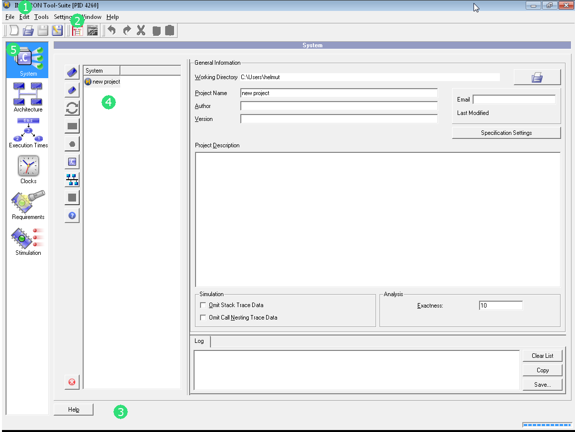
Figure 6.1: Areas of the Project Window #
Menu bar
Tool bar
Status bar
The module's input mask
Icon of the active module
6.1.1 Saving a System Model #
Tip:
Changes in the Project modules' input masks can be undone or redone with → and → or using the corresponding toolbar buttons.
The undo history is only limited by the computers main memory. The history is not reset on saving a project. On loading a project or creating new project using → the history will be deleted.
To permanently apply changes to a project it has to be written to disk with → .
Invalid or faulty project descriptions can only be removed by manually manipulating elements of your project file. This is done as follows:
Load the flawed project file.
Correct or delete the erroneous settings using the Tool-Suite GUI.
Finish your modifications by → .
6.2 Module System #
- 6.2.1 Concept of Module System
- 6.2.2 Adding and Removing System Elements
- 6.2.3 Drag & Drop and Copy & Paste
- 6.2.4 Project Information
- 6.2.5 Compiler And Preprocessor Options
- 6.2.6 Microprocessors
- 6.2.7 Peripheral Components
- 6.2.8 Add Source Files
- 6.2.9 Scheduler
- 6.2.10 Defining Processes
- 6.2.11 Modeling AUTOSAR Runnables
- 6.2.12 Modeling Process Dependencies
- 6.2.13 Event Chains
- 6.2.14 Rest Bus Model
For the following explanations please load the example project
examples/isr/bursty.ipr
and select the System module.
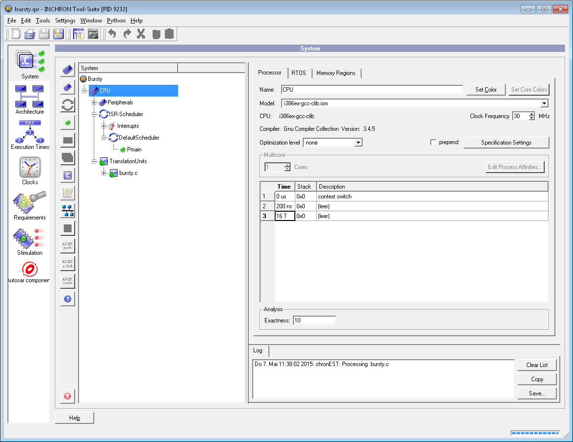
Figure 6.2: Module System #
6.2.1 Concept of Module System #
The module System presents the hardware and software aspects of the modeled system as well as mapping relations between these. The tree structure on the left show the model's processors as top level elements with assigned peripherals, schedulers, tasks and files as children. Elements may be moved by drag-and-drop mouse operations or copied using the clipboard. When reparenting items, INCHRON Tool-Suite will only accept valid combinations.
By ing a tree element an editable view of its properties will be shown to the right of the system tree.
Microprocessors are first order elements of an INCHRON project. Further first order elements of an INCHRON project are Event Chains (see Section 6.2.13, “Event Chains”) and RestBus (see Section 6.2.14, “Rest Bus Model”). A microprocessor has the following child elements:
- Schedulers
Each microprocessor has a root scheduler (ISR-Scheduler), which schedules ISRs and its Default-Scheduler. The Default-Scheduler schedules the processes mapped to the processor and optional sub-schedulers (hierarchical scheduling).
- Source Files
The processes running on a microprocessor execute entry functions of source files mapped to the same microprocessor.
Source files on project level may be used for function libraries. Using → INCHRON Tool-Suite searches the global source files for symbols (functions and variables), which are referenced in processes running on the microprocessor but unresolved by the processor's source files. As a result global source files containing such symbols will be added to the microprocessor.
- Peripherals
Peripherals (not peripheral buses) are also assigned to a microprocessor.
Peripherals have I/O ports for interconnection with ports of buses or other peripherals and interrupt (IRQ) ports which are subject to stimulation and which trigger interrupt service routines (ISR).
Event Chains appear as top level elements as the result of event chain instrumentation (see Section 6.2.13, “Event Chains”). Customizable settings of an Event Chain are custom step names and instance colors (used in simulation diagrams).
Elements representing peripherals, interrupt service routines, source files, and event chains are grouped by a Container Element. Their purpose is to allow collapsing of elements which are currently not of interest. The container elements are created and removed automatically. Except from grouping they have no functionality, especially there is no property widget associated with them. The source file container element shows the combined status of the contained elements as a hint.
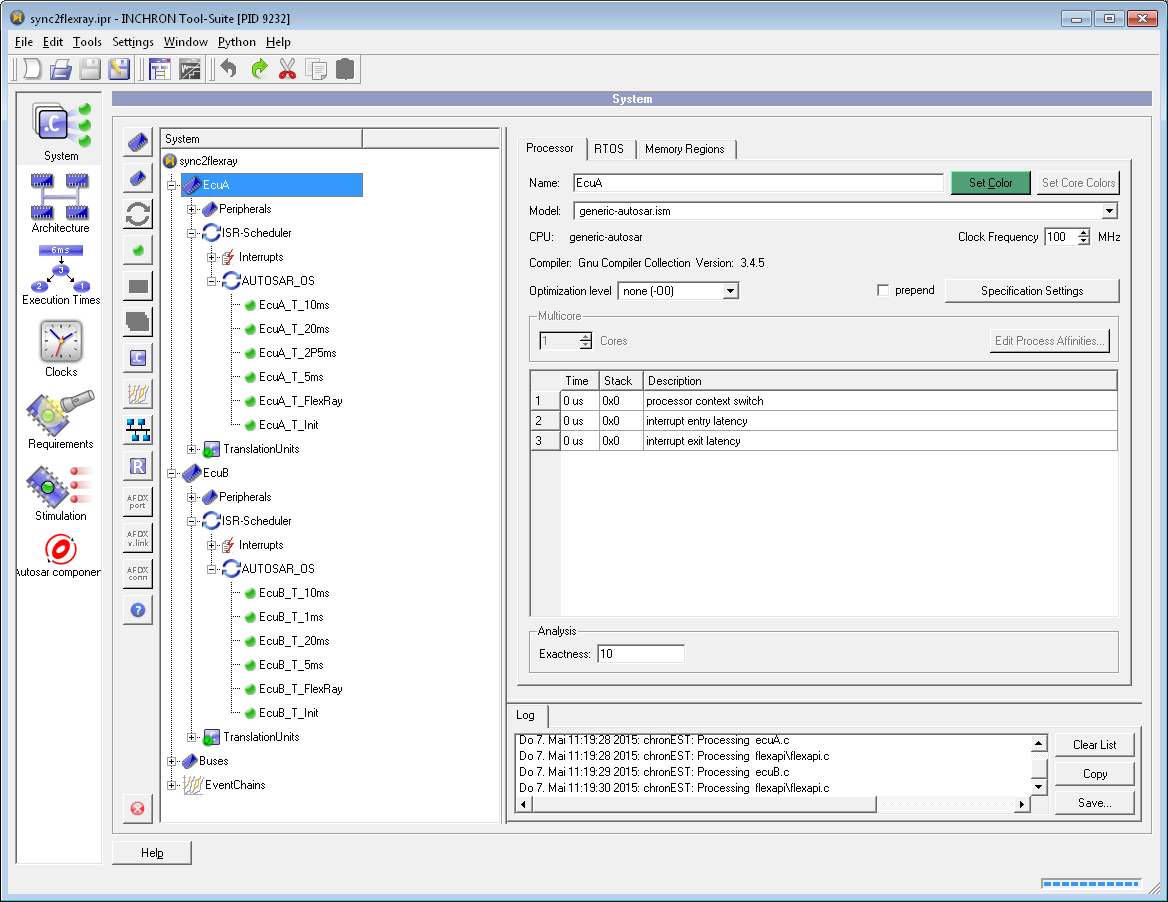
Figure 6.3: A typical system grouped by container elements, shown open and closed #
6.2.2 Adding and Removing System Elements #
The project element does always exist. To add a child element to any existing tree element do as follows:
 |
Deletion of an element will also delete all its children. |
Important:
Removing an element may imply further changes, e.g. removing a process may result in in a stimulation source loosing its stimulation target.
6.2.3 Drag & Drop and Copy & Paste #
The module System's system tree provides common GUI operations: Moving an element (and its children) may be performed by either drag & drop or using the clipboard (copy & paste). For clipboard operations the menu, the toolbar or the usual Ctrl–C and Ctrl–V keyboard combinations may be used.
6.2.4 Project Information #
Please select the root element (project) in the system tree of the System module.
The property view at the right of the system tree shows the project settings and information.
The following global project properties are shown:
Project status and
Project description
Working Directory
The project description may be used for documentation of simulation and analysis results and modification of project settings.
For the working directory it is recommended to use the root directory of the project's source files. In this case INCHRON Tool-Suite will save all file paths as relative path, which alleviates portability to other computers.
Figure 6.4: Global Project Properties #
It is recommended to save your current work before simulation,
analysis or before loading a different project.
6.2.5 Compiler And Preprocessor Options #
Compiler options and preprocessor definitions may be defined globally (on project), on each microprocessor or for each source file. For source file translation all options are concatenated in the following default order: project, microprocessor, source file. This default order may be modified for individual microprocessors and/or source files with a prepend option.
The settings dialog for each level is the same and offers three tabs for Include Path, Preprocessor Definitions and Compiler Options.
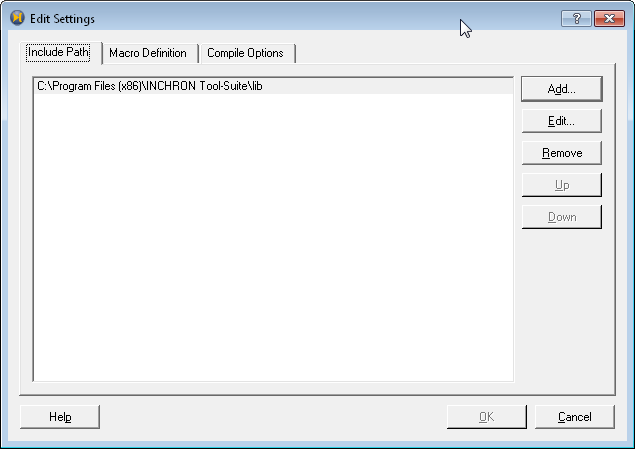
Figure 6.5: Include Path Settings #
6.2.5.1 Tab Include Path #
This tab allows to specify the directories where the compiler searches for header files.
From the system tree select the project, a microprocessor or a source file.
the button .
In the dialog Edit Settings select the tab Include Path.
The dialog wil now show the configured include paths as shown in the screenshot below.
the or button.
Choose an include directory and confirm with .
The include order may be changed with or .
Important:
The order of include directories defines is significant for successful compilation.
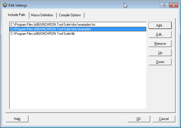
Figure 6.6: Global Includes #
6.2.5.2 Tab Macro Definition #
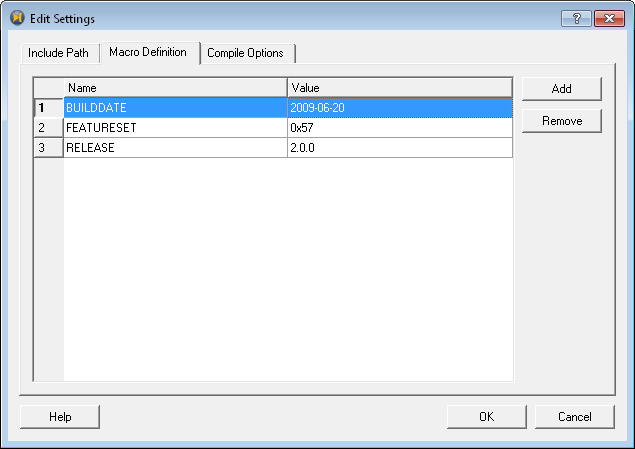
Figure 6.7: Global Macro Definitions #
Add definitions of required preprocessor macros and variables as follows:
button .
In the Edit Settings dialog select the tab Macro Definition.
to add an empty entry.
the cell in column Name to edit the macro name, and
the cell in column Value. Enter a macro Value as a valid ISO ANSI C expression in the context of the source files where the macro is compiled (the equivalent C macro definition
#define name valuemust be valid).Repeat steps 1 to 6 until finished.
Close the dialog by confirming with .
6.2.5.3 Tab Compile Options #
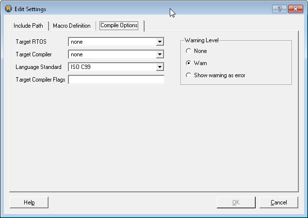
Figure 6.8: Compile Options #
For parsing of source files the OS type can be chosen
(for enabling special constructs like TASK(A) in case
of OSEK), as well as compiler, language standard and optimization switches.
With Warning Level the strictness of the compiler may be influenced: Warnings may be silently ignored or treated as errors. In case the compilation of a source file results with errors its item in the system tree will be shown with a red bullet and the generation of a simulation will not be possible.
6.2.6 Microprocessors #
6.2.6.1 Microprocessor Target Models #
Targets supported by INCHRON Tool-Suite are defined by a combination of
Supported microprocessors and operating system combinations are listed in Appendix A, Technical Data
This library of supported targets is subject to continuous extension by INCHRON.
A target can be chosen separately for each microprocessor of the system model:
Select a microprocessor in the system tree
Select the desired target from the Model combo box
6.2.6.2 Processor Properties #
Several properties of the target's microprocessor type may be adjusted. After selecting a microprocessor from the system tree its properties are shown distributed on three tabs to the right of the system tree.
6.2.6.2.1 Tab Processor #
This tab allows setting of basic microprocessor parameters. This includes the processor name, clock frequency, the used target model, a custom processor color and processor core colors used in diagrams. Additional settings are latencies of operations, preprocessor definitions and compiler options.
Figure 6.9: Microprocessor Properties #
6.2.6.2.1.1 Process States #
A target model also defines the variety of process states supported by the processor model.
- Dead (OSEK: Suspended)
The process is terminated.
- Ready
The process has been activated but not yet became running.
- Waiting (Blocked)
-
The process waits for release of a mutex, queue, semaphore, OSEK resource or a
resumeTask()after explicitsuspendTask()[1] . - System
-
The process is executing a system level operation like context switch (requires definition of a context switch cycle time).
- Running
The process is running.
- Preempted
-
The process has been preempted by a higher priority process. This state will be displayed as Ready in the Process State Diagram .
- Interrupted
The process has been interrupted by an ISR. For processor models not supporting this state this will be appear as Ready in the Process State Diagram.
- BusyWaiting
The process is executing a spinlock via
aquireSpinlock()(orGetSpinlock()for AUTOSAR models) or the BUSYWAIT_UNTIL() macro [2] or AUTOSAR synchronous wait for cross core interrupt. This state will be displayed as Spinlock in the Process State Diagram .
6.2.6.2.1.2 Setting the Core Affinity for all Processes on a Resource #
On multicore processors each process may be restricted to an individual set of cores. To edit these restrictions press . The Edit Process Core Affinities dialog opens and shows the current setting. If a checkbox is set the process is allowed to run on this core.
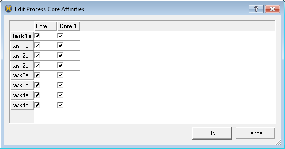
Figure 6.10: Edit Process Core Affinities Dialog #
Note:
If a new process is added, it is automatically enabled to run on all existing cores.
On the other hand, when increasing the number of cores, no process affinities will be enabled for the cores added. This means none of the existing processes will be allowed to run on added cores by default.
6.2.6.2.2 Tab RTOS #
The RTOS tab contains the maximum allowed number of tasks and latencies of the operating systems task operations. Attributes of the OS scheduler are configured at the scheduler element of the processor.
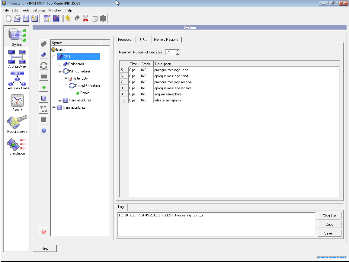
Figure 6.11: RTOS Properties #
6.2.6.2.3 Tab Memory Regions #
Each target's processor type has predefined memory regions (usually RAM and ROM). For your system model existing memory regions may be modified and more memory regions may be added.
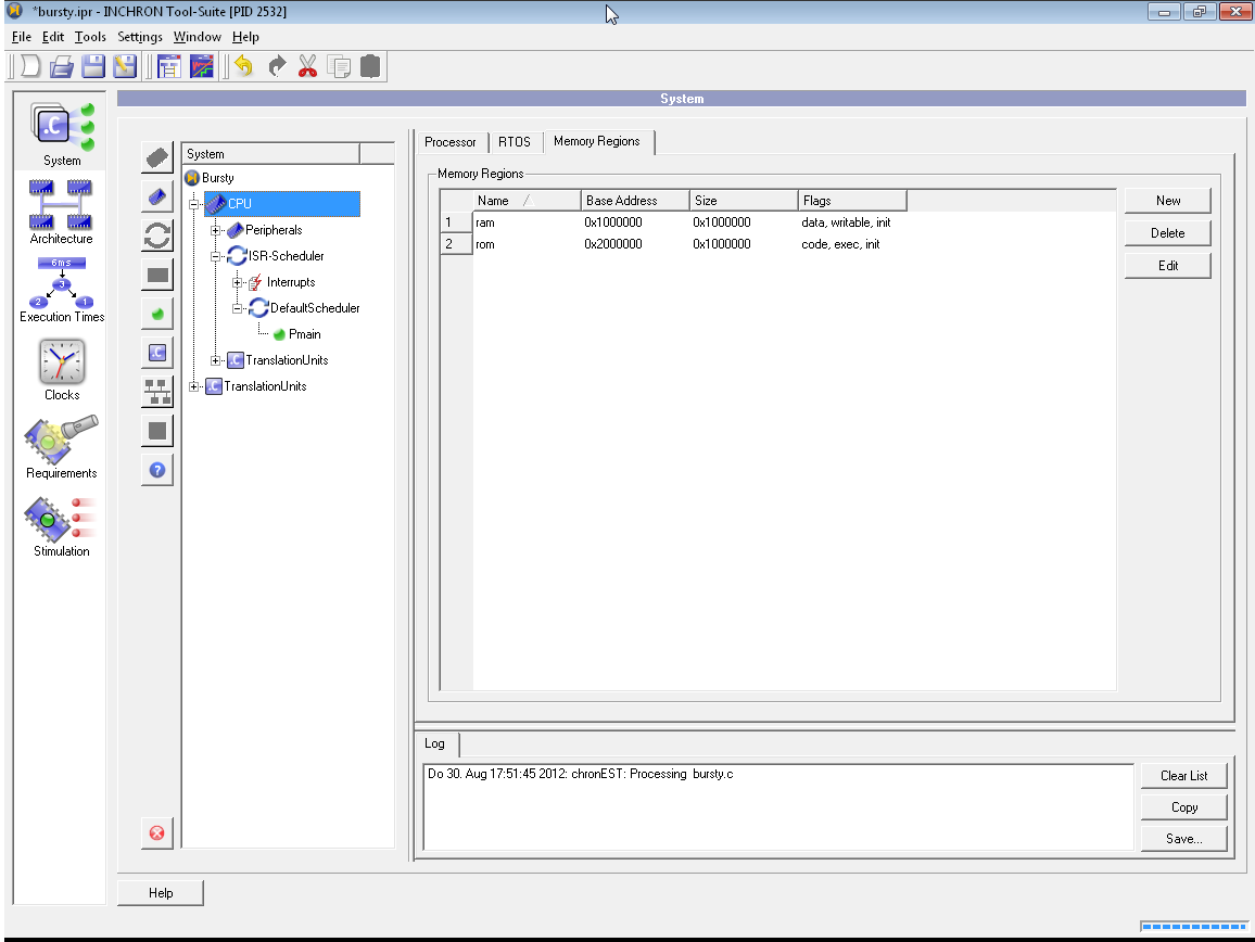
Figure 6.12: Memory Region Settings #
Configuration of a memory region requires the following settings:
The following additional flags are optional:
To change settings of a memory region select a memory region and the button.
The Memory Region Properties dialog pops up.
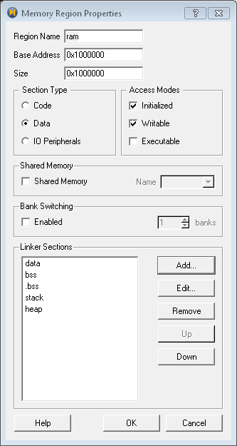
Figure 6.13: Memory Region Properties Dialog #
6.2.6.2.3.1 Shared Memory #
The Shared Memory option allows to use a
memory region to be shared between multiple microprocessors for
purpose of inter process (IPC) or inter processor communication.
If option Shared Memory is checked
Section Type Data will be selected
automatically and options not applicable are disabled.
A Shared Memory region may be mapped to different base addresses on different microprocessors.
The definition of multiple Shared Memory regions is possible. A Shared Memory region already defined may be selected for reference (or renamed) using the Name Combo Box.
6.2.7 Peripheral Components #
Peripheral Components are used to connect the microprocessors of the simulated system with each other and with the environment. The INCHRON Tool-Suite offers a set of predefined library models for them as described in Appendix C, Peripheral Components. These models focus on interaction with the processes by either a register set or a functional API, interrupt request lines (IRQ ports) for triggering interrupt service routines, and input-output ports for connections with other peripherals.
Peripherals come in two different types: buses which can be placed at the project level and controllers which can be placed at the microprocessor level. Currently the following set of peripherals is available:
The IRQ Source is the most simple form of peripheral component. It has a single port named IRQ which represents an input pin which triggers an interrupt when activated.
The Simple Input and Simple Output are plain 32bit wide ports which can be connected with each other. The Simple Input has an additional IRQ line which is triggered whenever data arrives.
The Simple UART models a serial transmitter/receiver. It can be connected only to other Simple UARTS.
A Simple Timer is driven by the clock frequency of the microprocessor it is connected to. After being started it counts down and triggers an interrupt when reaching zero.
SPI communication can be modeled by connecting a Master-SPI controller to one or more Slave-SPI controllers. In the Module Architecture the controllers can be daisy-chained. The SPI controllers offer a register set for usage in the simulated system.
CAN systems are supported by a Simple CAN Bus, a CAN Communication Controller, and a CAN Communication Controller (indexed), which has a configurable number of buffers accessible by an index. The controllers can be used by reading and writing a register set from the source code of the simulated system. Ask INCHRON about example code for a C library. A CAN bus is simulated on packet level, not on bit or physical level.
FlexRay systems are also supported by a FlexRay Bus, and by a set of FlexRay controllers. While the Flex4200 FlexRay Communication Controller and the Bosch E-Ray FlexRay Communication Controller emulate the register set of their archetype the Simple FlexRay Communication Controller can only be accessed by a functional API.
The Simple LIN Bus is used to model a LIN system. It can be combined with a LIN Communication Controller, which is accessible by a functional API.
Ethernet systems are supported by an Ethernet Switch, which has scalable number of ports, and a Generic Ethernet Controller with a functional API. It only supports switched ethernet with point-to-point connections. For each link full-duplex or half-duplex, and its speed can be selected.
Some microprocessor models like the nev-v850-pho3 or the m16c60 come with predefined peripherals. These peripherals do appear automatically as children of the microprocessor in the system tree. Additional peripherals may be added at any time during modeling.
To be used in a simulation, each peripheral usually requires the definition of a non-conflicting base address and port connections to other peripherals.
A peripheral is added as follows:
-
Select a processor in the system tree if you want to add a controller peripheral. Select the project if you want to add a communication bus.
in the toolbar left to the system tree.
The Add Peripheral Component Dialog opens.
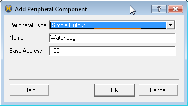
Figure 6.14: Selection of Peripherals #
Select a Peripheral Type
-
Enter a unique Name and, if required, a Base Address.
The base address defines the address for accessing the peripherals registers and must be uniq. In case of a conflicting address the dialog cannot be confirmed.
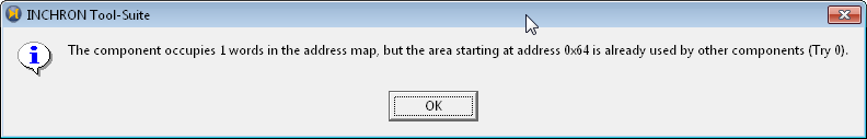
Figure 6.15: Error Message on Address Conflict #
Confirm your settings with .
Repeat steps 1 to 5 until finished.
If a peripheral in the system tree is selected its properties are shown on the right. The number and type of the properties depends on the type of peripheral. See Appendix C, Peripheral Components for more information on the peripherals.
For visualization and editing of the connections of input and output ports use the connection editor of Module Architecture. Configuring the association of interrupt ports (named IRQ) with interrupt handlers (ISRs) is available as part of the properites of individual ISRs.
6.2.7.1 Modeling Bus Messages #

The peripherals of type CAN Communication Controller, CAN Communication Controller (indexed), Simple FlexRay Communication Controller, and Generic Ethernet Controller also offer the possibility to model the transmission of data frames in system models without source code. These peripherals have a Message Scheduler to which the messages are added.
The properties of a message can be edited by selecting it.
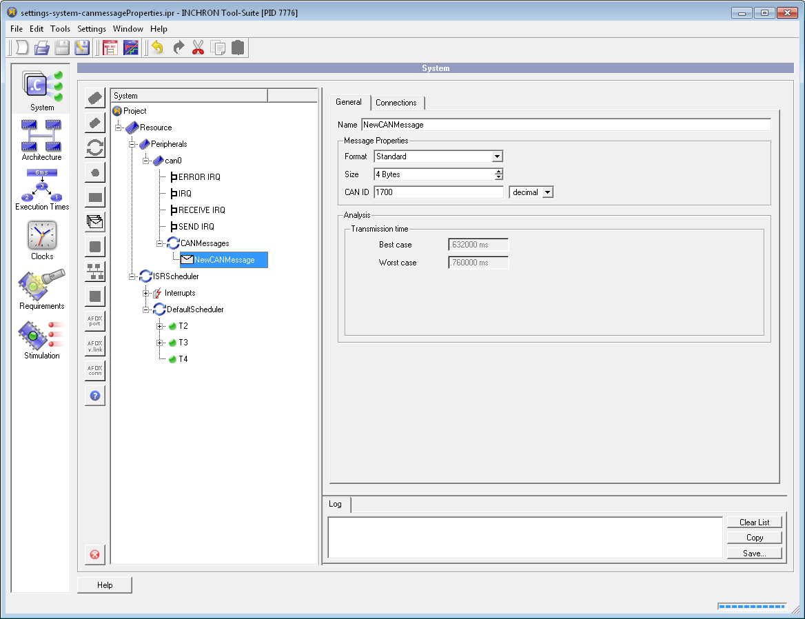
Figure 6.16: Message Properties #
The parameters of a message depend on the type of peripheral component.
Important:
For a Simple FlexRay Communication Controller running as a SYNC node or as a coldstarter at least a FlexRay message is required with the same id as selected for the pkeyslotid.
6.2.8 Add Source Files #
The same source file may be added to multiple microprocessors on project level and show up as individual tree element with individual source file settings. On the other hand, changes to a source file may affect the simulation of different microprocessors if multiple system tree file elements reference the same file.
A source file is added as follows:
In the system tree select a microprocessor or the project.
the
 source file symbol in the toolbar on the left of the system tree.
A file dialog opens.
Select one or more source files to be added and confirm with .
For each new source file, a new file child element will be shown. The source file will automatically be parsed and the source file icon will indicate the compilation status in
 green or
  red.
On success, function child nodes will be added accordingly.
red.
On success, function child nodes will be added accordingly.
If files added to the project are located below the project's working directory (see Section 6.2.4, “Project Information”), Tool-Suite will save relative paths in the project file. This facilitates relocation of INCHRON projects and portability between different computers. Thus it is recommended to always set a project working directory.
Selection of a file element will show its properties and settings. These are the name of the element (which is the source file's path name relative to the project's working directory), the file's Specification Settings and compiler messages resulting from parsing the source file.
6.2.8.1 Supported C-Code-Standards #
INCHRON Tool-Suite supports ANSI C standard according to Brian W. Kernighan & Dennis M. Ritchie, published by the ANSI committee X3J11 as ISO C, including amendment 1.
6.2.8.2 Supported File Extensions #
By default INCHRON Tool-Suite accepts only files of the type .c as C source code,
and .cpp as C++ source code.
If there are other file extensions that should be accepted as C or C++ source code,
they can be entered using the Tool Settings dialog
(see Section 4.4.1.2, “Source Code File Extensions”).
These file types will then be available in the File Open dialog filter option.
6.2.9 Scheduler #
In order to assign processes to run on the cores of a microprocessor a scheduler is required. The algorithm to assign CPU time to processes is defined by the scheduler type and strategy.
The DefaultScheduler which is automatically assigned to each microprocessor of an INCHRON Tool-Suite system model contains the processes to be run on the microprocessor.
DefaultScheduler is always child of an ISR-Scheduler which schedules the microprocessor's interrupt service routines. The ISR-Scheduler is priority based so that ISRs will preempt the processes of the DefaultScheduler.
The default type of the DefaultScheduler depends on the chosen operating system.
Note:
POSIX scheduling can be approximated via a time-sliced fixed priority scheduler and identical priority levels.
INCHRON Tool-Suite supports the Hierarchical Scheduling concept. A sub-scheduler added to a given scheduler shares the time budget assigned by its parent scheduler among its child processes according to its strategy.
A scheduler may be added as follows:
Select a microprocessor's ISR or default scheduler.
Add a Scheduler using the shown
 button or via context menu and select it.
The scheduler properties are shown to the right of the system tree as in the screenshot below.
Configure the scheduler.
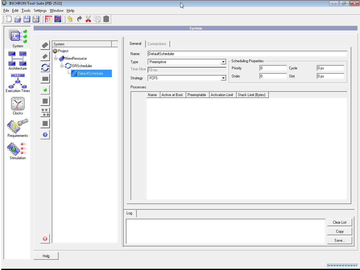
Figure 6.17: Scheduler Properties #
Select a scheduler Type to define when scheduling of a process takes place. The type Time-Slice has an additional parameter for the duration of the time slice. With Strategy an algorithm is chosen for the selection of a process to be scheduled.
The Scheduling Properties group box shown in Figure 6.17, “Scheduler Properties” is disabled for a microprocessor's root scheduler (ISR-Scheduler). For a sub-scheduler it shows the same scheduling properties as shown for processes.
The system tree in Figure 6.20, “Process Properties” shows a scheduler with two processes and one sub-scheduler with two more processes. The Processes table in the same figure lists the scheduling parameters of the scheduler's children.
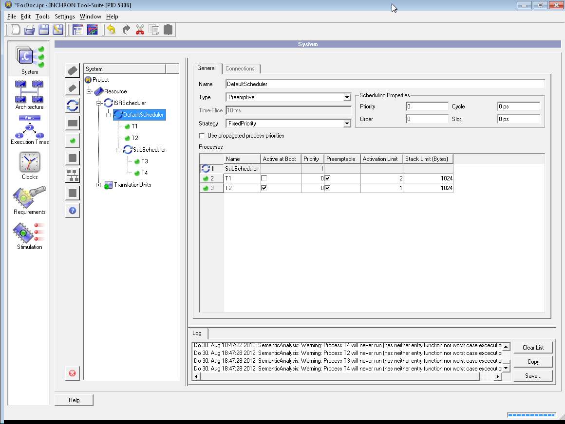
Figure 6.18: Scheduler with two processes and a sub-scheduler #
6.2.9.1 TDMA Scheduler #
A TDMA scheduler assigns a fixed amount of time to each of its processes. This amount of time is called a slot. If the process is active it can run only in the specified slot. When the slot ends the process is preempted. If no slot is active within a slot the processor stays idle. When all slots have been processed the whole cycle starts anew. Besides processes also sub-schedulers can be managed by a TDMA scheduler.
The Scheduler Property Widget for a TDMA scheduler differs from the one for other schedulers: The TMDA scheduler can have identical entries at different positions. This does not make sense for e.g. a fixed priority scheduler. The following figure illustrates this.
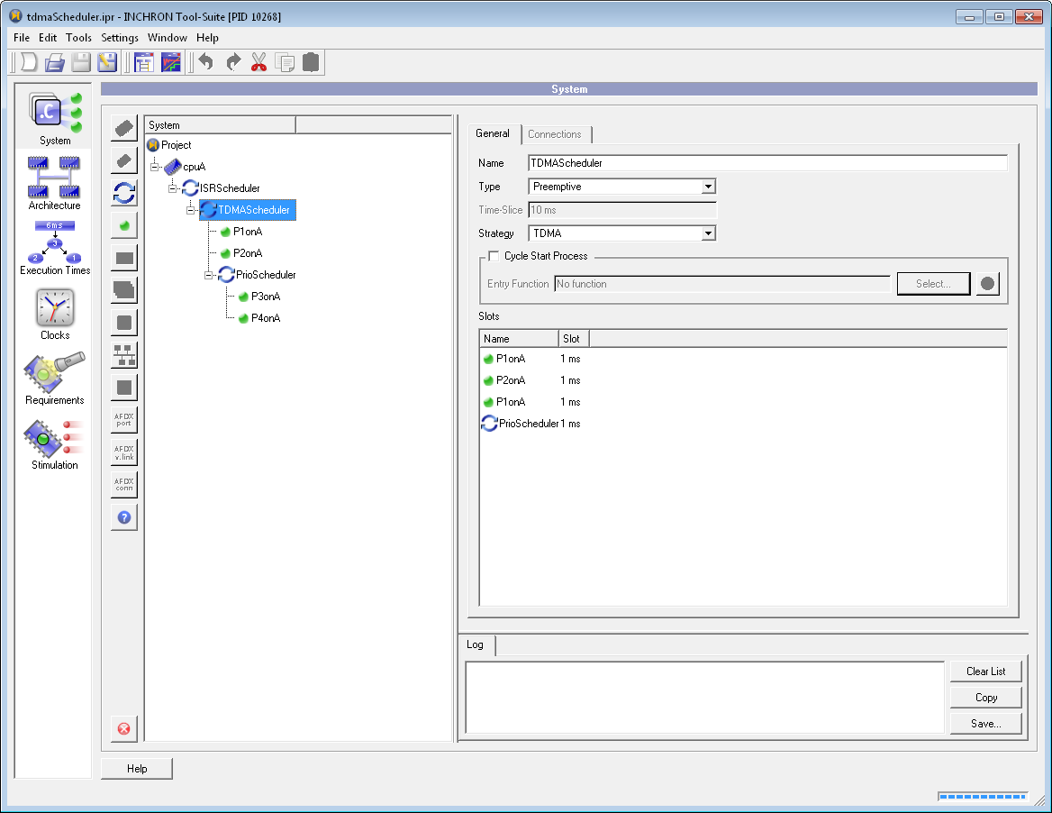
Figure 6.19: Property Widget of a TDMA Scheduler #
The figure shows a TDMA scheduler having two processes and one priority scheduler as direct descendants. The schedule starts with process P1onA, it can run for 1ms. Process P2onA is scheduled next for 1ms, too. Then P1onA gets the processor again for another 1ms. At the end of the cylce an identical slot of 1ms is assigned to PrioScheduler, which selects the highest priority process from P3onA and P4onA which is active. Afterwards the schedule starts again with P1onA.
The schedule of a TDMA scheduler can be edited as follows:
New entries can be added to the table by selecting the TDMA scheduler in the system tree and then using drag and drop to move processes or sub-schedulers into the list of slots. A blue line shows where the element will be inserted.
The slot duration can be changed by first selecting the entry and then clicking into the time value. A time value consisting of a number and an unit has to be entered. The data entry has to be finished by pressing Return.
Entries are removed from the slot list by selecting the entry and then pressing Delete.
The order of the entries can be changed by drag and drop within the slot list. Again a blue line will show where the entry will be placed. As usual pressing Shift or Control during the drop will switch between moving the entry and inserting a copy.
Processes and sub-schedulers can be placed several times in the list of entries. This can be done by using drag and drop either from the system tree or within the list while pressing Control.
Only items which are direct descendants of the TDMA scheduler can be placed in the slot list. Also every child has to be placed in the slot list at least once. This limitation may be removed in future releases.
A slot length of zero (0s) is allowed, the corresponding entry will receive no processor time at all. To add an empty slot (e.g. for reserving processor load for future system components) define a dummy process which will never be activated and add it to the slot list with the desired slot length. The total cycle length of the TDMA scheduler is calculated automatically.
6.2.10 Defining Processes #
The properties view of a scheduler lists its child processes. The following steps describe adding and configuration of a process. For defining an ISR (Interrupt-Service-Routine) the same steps have to be performed on the ISR-Scheduler of a microprocessor:
Select a scheduler.
Use from the context menu or click the corresponding
 button.
A new process child is added to the scheduler.
Select the new process.
The process properties are shown as in the screen shot below.
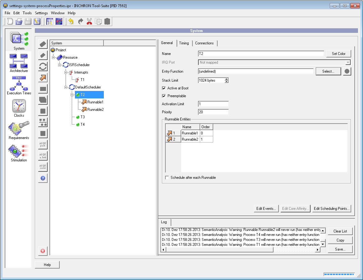
Figure 6.20: Process Properties #
6.2.10.1 Process Properties #
The properties of a process (or ISR) or a basic or extended task in case of OSEK or AUTOSAR are divided on the three tabs General, Timing and Connections.
6.2.10.1.1 Tab General #
Name of the process.
With a custom color to be used in diagrams may be chosen.
In case of an ISR, the peripheral interrupt port (named IRQ in the Architecture Module) which triggers this ISR can be chosen from the IRQ Port drop down list.
Entry Function selects the process entry function. When clicking on (or just the text field to its left) the Object Selection Dialog opens, showing all available functions of the CPU resource.
The defined Stack Limit of a process defines how much stack will be reserved for the process. This must not be confounded with the expected Stack Usage which is defined on Timing tab.
Active At Boot, Preemptable and Activation Limit define basic scheduling properties of a process which are used independently of the used scheduling scheme.
Often a CPUs has one or more idle task which shall be excluded from evaluations. By marking a process as Idle Task it will
be excluded from load calculations (in the Statistics View and Load Diagrams),
not be evaluated by reporting functionality and
initially be hidden in Process State Diagrams.
The Priority of the process is only used (and editable) when the process is managed by a priority scheduler.
Additional Properties for OSEK and AUTOSAR Modeling #
The following options on Tab General are available for OSEK and AUTOSAR processor models only:
Switching the OSEK Task Type (either basic or extended task) will adjust the columns available for activation of runnables (with either cyclic or event based triggering) of the Runnable Entities table accordingly.
For AUTOSAR models a table of Execution Blocks will be shown (see Section 6.2.11.1, “Execution Blocks”)
The button will show a dialog for defining OS (OSEK) events. These are the relevant events to be associated with Execution Blocks in order to trigger the execution of AUTOSAR runnable entities.
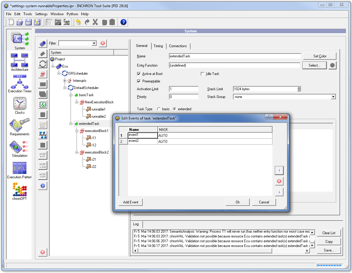
Figure 6.21: Edit Events Dialog for a task #
The button will show a dialog for defining a sequence scheduling points.
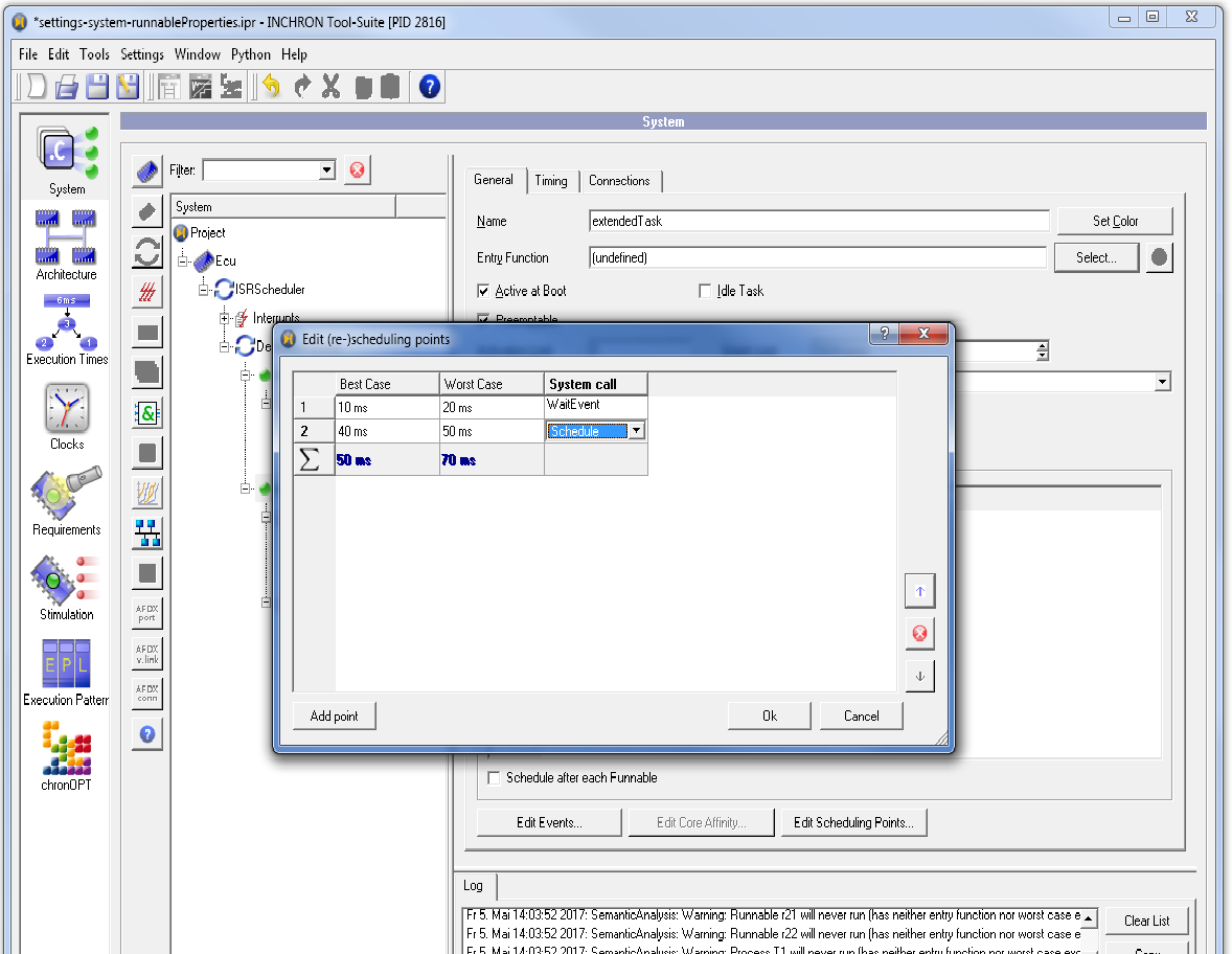
Figure 6.22: Edit Scheduling Points Dialog #
6.2.10.1.2 Tab Timing #
The Tab Timing is for specifiyng certain timing parameters most notably best and worst case execution time (BCET, WCET) and for defining a replacement timing behavior of a process for a task model where neither Entry Function nor Execution Blocks (i.e. runnables) have been defined for the process.
Best Case and Worst Case on tab Timing are for specifying execution times. These are evaluated by chronVAL validation or for chronSIM simulation with task models (i.e. in case of neither entry function nor runnables have been specified). Wether and how the given values for best and worst case execution time are applied is controlled by the selected Simulation Replacement option (as follows).
With Simulation Replacement on tab Timing the simulation of randomly distributed execution times may be configured. These Simulation Replacement does apply for chronVAL analysis or chronSIM simulation of task models (i.e neither an entry function nor runnables are specified for the process). Uniform and normal distributions are suppported. In both cases the values of BCET and WCET have the role of constraints.

Important:
This means when specifying Normal distribution, the Worst Case input field must not be empty or the resulting execution time will always be
0 msdue to the imposed constraint.Blocking Time on tab Timing is used for chronVAL validation to define a maximum time a process is waiting for resources.
if a process has no entry function defined, its timing behaviour is derived from BCET, WCET and the simulation replacement (see above). In the same way the Dynamic Stack Usage on tab Timing of a process defines how much stack the process uses at runtime.
With the Call Nesting parameter the simulated call nesting increment per function call for that process can be set.
6.2.10.1.3 Tab Connections #
Another way to induce the invocation of a process (or a runnable) is via outgoing connections of the dependency graph . The semantic of a connection is that the termination of the source process will trigger the activation of the target process. Connections can be added by just dragging any process in the System tree to another one (in the same tree view). In case source and destination are not visible at the same time in the tree view, the Connections tab just facilitates to connect a source element from this secondary tree view to the main tree view.
Important:
Outgoing connections are always triggered, independently of the definition of a process entry function for the process.
6.2.10.2 Setting the Core Affinity for a Process #
On multicore processors each process can be bound to an individual set of cores. To change this press . The Edit Core Affinity dialog opens and shows the current setting. If a checkbox is set the process is allowed to run on this core.
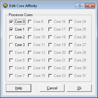
Figure 6.23: Edit Core Affinity Dialog #
Important:
When changing the number of cores, no process affinities for new cores added. This means that existing processes are not automatically allowed to run on new cores. On the other hand if a new process is added it is automatically allowed to run on all existing cores.
For convenience the core affinities of all processes can be edited at the same time with the Edit Process Core Affinities dialog of the resource properties.
6.2.11 Modeling AUTOSAR Runnables #
On a CPU resource with an AUTOSAR processor model any process modeled represents either a Basic Task or an Extended Task (in terms of the OSEK standard). As runnable entities may be triggered by different RTE events, groups of runnables to be executed by the same event are comprised in so-called Execution Block containers at a process (task).
-
A Basic Task always has a single Execution Block which is triggered by process activations.
-
An Extended Task has one or more Execution Blocks, each being associated with an OS event (which is defined via of an extended task) for triggering the execution of its sequence of runnables.
-
In case of a process on an AUTOSAR CPU, neither its entry function is called nor is the timing behavior applied as defined by the Simulation Replacement. Instead, only the specified behavior of individual runnables being executed determines the timing behavior of the process. Defining the behavior of a runnable is analogous to that of a process (see Section 6.2.10.1, “Process Properties”), i.e. by specifying either a Simulation Replacement or an entry function.
In order to define an Execution Block and its runnables, do as follows:
-
Select a
process by clicking it.
-
Click the
 Add Execution Block tool button.
-
Click the
 Add RunnableEntity tool button as many times as needed.
Note:
In case an entry function is defined this will take precedence over both the definition of Execution Blocks and the definition of Simulation Replacement (on tab Timing).
In case at least one Execution Block is defined this will also take precedence over the definition of a Simulation Replacement.
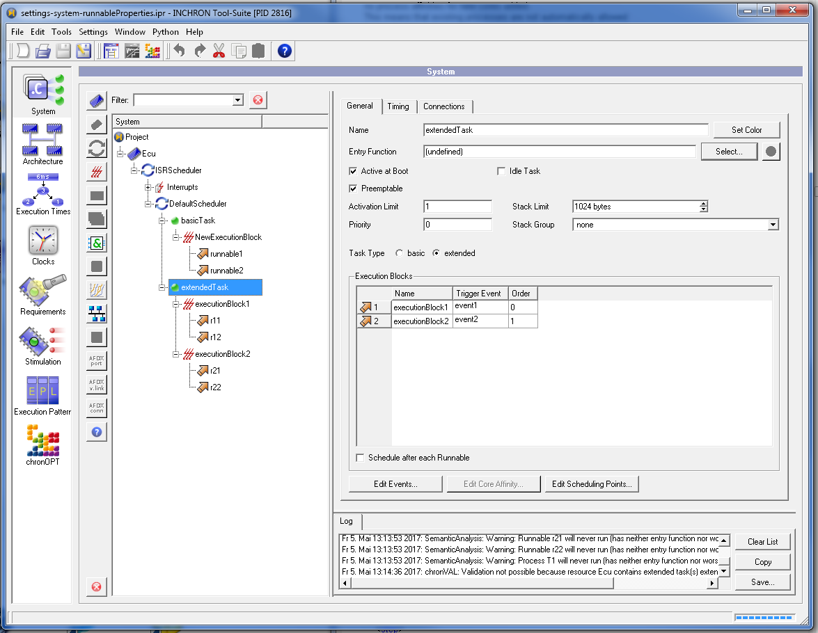
Figure 6.24: Extended Task with Two Execution Blocks #
6.2.11.1 Execution Blocks #
All defined runnables of an Execution Block are summarized in a table shown with the process properties.
In case of an extended task an execution block to be triggered has to be associated with an OS event. This can be set or edited as either the OSEK Event at the execution block or as Trigger Event in the Execution Blocks table in the process properties.
In case of a basic task
the Execution Blocks table will take no more than a single entry.
the relation of task activation and actual execution of the sequence of runnables depends on the parameters Offset and Cycle of the Execution Block. I.e. with parameters Offset = 5 and Cycle = 2 the first execution of the Execution Block will be with the 5th activation of the task and subsequently on every second task activation.
The order column defines the order in which the runnables are executed in the context of the execution block. Values for order can be edited in place in the table in order to define a different execution order for the runnables. The Schedule after each Runnable option controls if a cooperative scheduling point shall be inserted after the execution of a runnable.
6.2.11.2 Modeling Runnables with non-AUTOSAR Models #
The modeling of AUTOSAR runnables is also supported by non-AUTOSAR processor models (ISM), i.e. the generic-* models and its variants but not by the *-osek models.
For these processor models no Execution Block
element will be displayed.
All defined runnables of a process are listed in a table on the
tab General of the process properties.
This means when in case of non-AUTOSAR models,
processes may just be modeled as basic tasks aggregating runnable entities.
When you select a process by clicking it,
the Add Process tool button changes to
Add RunnableEntity.
Clicking it adds a runnable to the selected process.
In case a process has runnables, neither its entry function is called nor is the timing behavior applied as defined by the Simulation Replacement. Instead, only the specified behavior of individual runnables being executed determines the timing behavior of the process. Regarding timing and behavior, each runnable can be modeled just like processes, i.e. by specifying WECT, BCET, etc. or alternatively an entry function from a C source code module.
The column order defines the order in which the runnables are executed in the context of the process. Change this value to define a different order.
The checkbox Schedule after each Runnable selects if a cooperative scheduling point is inserted after the execution of a runnable.
6.2.11.3 Triggering the Execution of AUTOSAR Runnables #
The execution of the sequence of runnables of a basic task is triggered by activations of the containing process. Currently triggering the execution of runnables of an extended task is supported in two alternative ways:
A sequence of runnables can be targeted by an OS Event by selecting it from the OSEK event list of their Execution Block. In case of a basic task the execution depends on the parameters Execution Block.
OS Events can be defined (or removed) via the of the process properties of an extended task.
Individual runnables can be targeted by a stimulation generator.
6.2.11.4 Properties and Behaviour of a Runnable #
The properties of a runnable resemble in most aspects the properties of a process. Especially modeling the timing behavior of a runnable is mostly equivalent to that of a process. The properties can be edited by selecting the runnable.
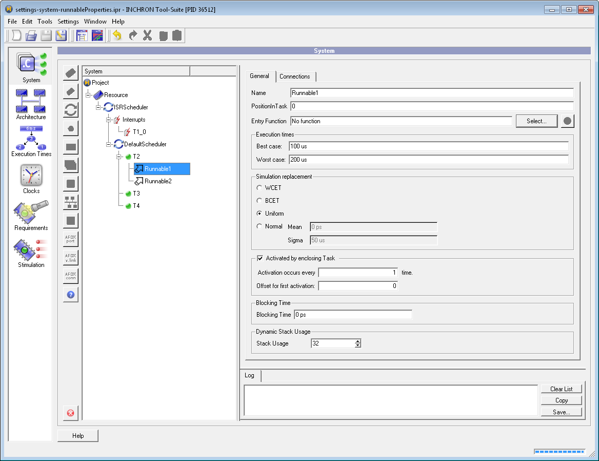
Figure 6.25: Runnable Properties #
A runnable has the following properties:
Name of the runnable.
Position in Task corresponds to the execution order of the runnable within the enclosing task.
Entry Function selects the function which is executed during simulation. This can be undefined to make the Simulation Replacement settings take effect.
Best case and Worst case define the execution time of the runnable. It is used in chronVAL and in a simulation when no entry function is defined.
For runnables without an entry function the simulation behavior can be defined modeled with the Simulation Replacement
If a runnable has no incoming connections (see Section 6.2.12, “Modeling Process Dependencies” for details) it is activated every time the enclosing task is executed. With the fields in the group Activated by enclosing Task this can be narrowed to a period and offset divider.
Blocking Time is used for chronVAL validation in order to define a maximum time a process is waiting for resources.
Stack Usage defines the amount of stack a runnable uses during execution. In the simulation it is added to the current stack usage of the enclosing process and all runnables.
6.2.12 Modeling Process Dependencies #
With INCHRON Tool-Suite, process dependencies are defined by bilateral process activations and communication in the simulation model's source code which are executed during simulation. For system models without source code an alternative mechanism for defining this kind of process dependencies is required since the source code is not subject to chronVAL validation. This is the purpose of incoming and outgoing elements which define the edges of a process dependency tree.
Incoming and outgoing elements may be added to processes of an INCHRON project as follows:
In the system tree select e.g. the process T1 and then the Connections tab in the process property view.
The Connections tab shows a tree view of target processes.
Select e.g. process T2 from the tree of dependency targets and press
As result, in the system tree the selected target process will be added as Incoming child of the process T2 and T2 will be added as Outgoing child of the target process.
Accordingly when selecting target T3 and pressing Add Outgoing the target will be added as an Outgoing child of the process and the process will be added as Incoming child of the target process.
The following image shows the resulting dependencies.
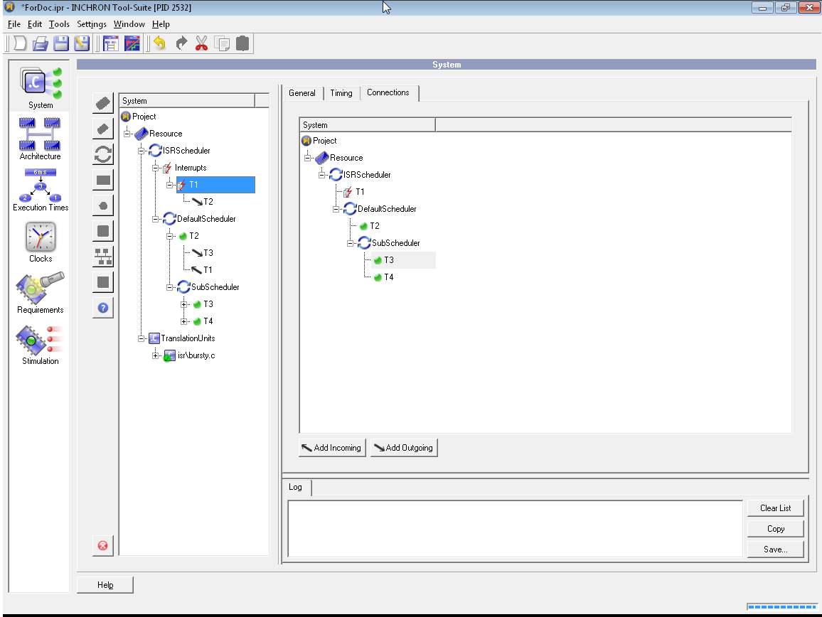
Figure 6.26: Process Dependencies #
Dependencies can not only be defined between processes or interrupt services routines, but also between processes, runnables and bus messages, and vice versa. When a bus message has an incoming dependency from a process it is scheduled for transmission. The transmission itself uses always the scheduling of the bus connection, e.g. priority arbitration for CAN or TDMA scheduling for FlexRay.
A dependency has properties itself, too. A group of Activations parameters allow the specification of a period and offset based divider. Additionally a dependency can represent Dataflow instead of activating the receiver. For the Communication Type a selection between Queuing, Shared Variable and Event based is possible. A Queue Length can also be specified. Especially for queued communication a checkbox Consume All selects that all data is read from the queue in a single execution of the receiver. These parameters specify how the event chain tokens are propagated along the dependency.
When there a multiple Incoming dependencies for a process each one activates the process. A logical AND Dependency can be added instead to express that all Incoming dependencies are needed to activate the receiving process.
Apart from mutual process activation, tasks may be triggered by external stimulation (see Section 6.7, “Module Stimulation”) from external ports.
6.2.13 Event Chains #
For the following explanations load the example project CanGateway\Gateway.ipr.
Event chains are a means for dynamic data flow analysis with chronSIM. An event chain in a chronSIM system model comprises a repeatedly occurring sequence of processing steps. These steps represent a causal chain, where the dependency between consecutive steps is characterized by e.g. a producer-consumer relation or an input-output dependency. A typical use case for an event chain is a processing pipeline in a sensor-processor-actuator system, By using event chain instrumentation on the simulation models source code, it is possible to track the succession of data entities through such processing chains during simulation with chronSIM. The simulation records one or more such dependency chains for later analysis using diagrams or real-time requirements.
Sequences of event chain steps emitted during the simulation define a graph of consecutive processing steps. Event chain instance graphs are visualized in the Event Chain Diagram, the State Diagram and the Sequence Diagram.
For a detailed introduction to the usage of the event chain API refer to the application note Reference Manual of Macros and Functions which is available via the Tool-Suite's help menu.
6.2.13.1 Event Chains Settings #
In contrast to the EVENT() macros which only affect the simulation trace,
event chains defined by DECLAREEVENTCHAIN() macro calls also
appear in the project editor's system tree
as children of the project node and allow custom settings,
which influence the event chain graph appearance in diagrams.
The following image shows the editable properties of an Event Chain:
A symbolic name may be assigned to the steps of an Event Chain. The names will be used instead of step numbers in diagrams which show Event Chains.
For distinguishing consecutive invocations (instances) of an Event Chain flow a palette of instance colors may be defined.
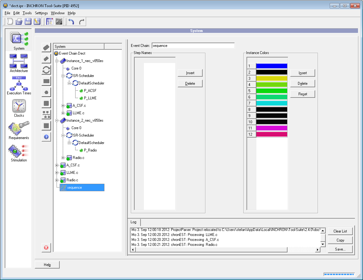
Figure 6.27: Event Chain Properties #
Assigning symbolic names for the steps of an Event Chain is done as follows:
Press the button of the Step Names group.
A new row with empty name column will be shown. Step numbers are shown on the left.
in the empty name cell, enter a step name and confirm with .
Selected names and colors may be discarded with the button.
Accordingly Event Chain instance colors may be added or removed with the and buttons of the Instance Colors group. A color dialog is invoked by an existing color entry. With the button the default palette is restored.
If during simulation an event chain flow is invoked (instantiated) more often than the number of defined colors then the defined colors are applied repeatedly in the same order.
6.2.14 Rest Bus Model #
In order to facilitate testing of a system model in a realistic environment INCHRON Tool-Suite allows a combined simulation of the system model with a chronBUS rest bus model. This allows for simulation of the real-time behavior of systems with CAN- and FlexRay controllers on buses with realistic workloads.
For this purpose a rest bus model is added to the project The rest bus model represents an ECU network which generates bus workloads. The ECUs of the rest bus are not visible in the system model. On the other hand CAN and FlexRay buses to be interfaced with the system are accessible in the system tree.
The buses parameters, ECUs and messages of the rest bus models may be modeled in detail. To model drift effects the rest bus ECUs have their own (drifting) clocks. The time jitter of messages sent by the rest bus simulation can be adjusted separately for each rest bus ECU.
6.2.14.1 Rest Bus Creation #
For adding an empty chronBUS model to a INCHRON project select either the Module Architecture or the Module System and press the button.
A rest bus will be added to the project element of the system tree.
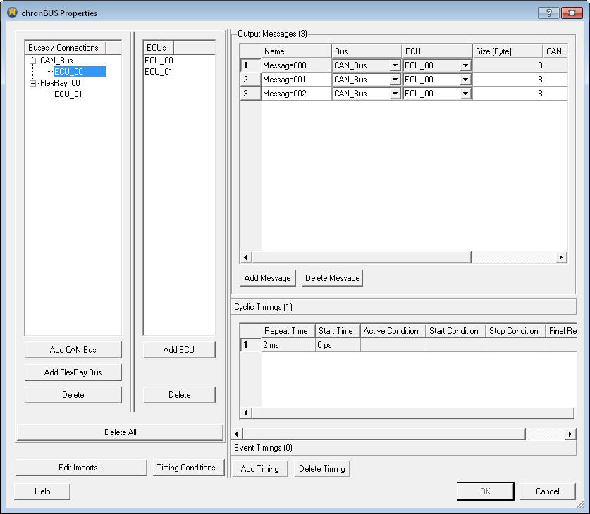
Figure 6.28: Module Architecture With Rest Bus #
6.2.14.2 Rest Bus Structure #
A chronBUS rest bus model consists of the following elements:
Buses and ECUs: A rest bus model contains one or more buses (CAN and/or FlexRay) as well as ECUs, which send messages on these buses.
Bus ECU Connections: A connection between an ECU and a Bus is required, if an ECU sends messages on this bus. ECUs of the rest bus do not model the reception of messages. ECUs of the rest bus model may be connected to buses in the same way like ECUs of the system model, no matter whether these buses are part of the system model or of the rest bus model.
Messages: For each Bus ECU connection one or more messages to be sent are defined. The message content of rest bus messages (signal structure of the message frames) will not be modeled.
Message Timings: The send time of bus messages is defined by message timings. The following timing types are available:
Cyclic Timings for CAN and FlexRay buses
Absolute Scheduled Timings for FlexRay buses
Event Timings for CAN and FlexRay buses
On FlexRay buses only Absolute Scheduled Timings are of functional relevance. Their Cyclic Timings and Event Timings are only descriptive for the rest bus model.
Timing Conditions: Cyclic Timings and Absolute Scheduled Timings may be controlled by optional Timing Conditions.
Elements of the rest bus model may be added and removed.
Alternatively system descriptions of ECU Controller networks and signals may be imported into the rest bus model directly from FIBEX or DBC files. The import of multiple DBC or FIBEX files is possible.
The resulting elements of a rest bus model may be edited after import. When saving the INCHRON project to an IPR file the rest bus model is saved together with the system model.
The following section describes the creation, configuration and use of a rest bus model.
6.2.14.3 Rest Bus Example #
The following descriptions are based on the INCHRON example project
Restbus.ipr from the directory doc\examples\Restbus
which already contains a rest bus model.
The projects system model contains two ECUs
Tester and Ecu, which each have a CAN controller connected.
The CAN controllers are connected by means of a CAN bus.
On both ECUs an OSEK OS is running.
Both ECUs each have three tasks, which are implemented in the
source files Ecu.c and Tester.c:
a startup task and two tasks and ISRs for sending and receiving of CAN messages.
ECU Tester periodically sends a message with CAN ID 2000 every
50 ms to ECU Ecu, which is
responded after 5 ms with a CAN ID 2001 message.
The rest bus model contains one ECU which sends three messages with CAN IDs 0, 1 and 2 of high priority
and of periodicities 2 ms, 4 ms and 10 ms.
The rest bus ECUs are modeled with no clock drift and jitter.
The periodicity of the message sent by the Tester jitters with max. 0.1 ms.
6.2.14.4 Rest Bus Configuration #
After loading the project the dialog for editing the rest bus model may be opened by on the rest bus element in the system tree. The RestBus Properties dialog shows
a bus connection tree and
an ECU list on the left and
a wider list for Bus Messages on the right top.
An additional property view on the bottom right displays either bus, ECU or message properties depending on the selection of either a message, an ECU or a bus in one of the lists.
The bus connection tree on the very left shows all buses of the rest bus model and the connected ECUs. ECUs may be connected to a bus by just dragging them from the ECU list to a bus of the bus connection tree.
The table Output Messages on the right top shows all messages sent by the bus ECU connections selected in the tree view.
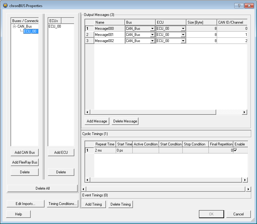
Figure 6.29: Rest Bus Configuration Dialog #
The GUI of the rest bus dialog mirrors the hierarchical relations of the rest bus elements:
In order to view the properties of a Bus/ECU combination, select one ECU connection in the bus connection tree.
In order to populate the message view, select one or more ECU connections in the bus connections tree. Alternatively you may select a bus, to show all messages of all connected ECUs.
In order to view the properties of a bus, select the bus in the bus connection tree view.
In order to view properties of an ECU, select an ECU in the ECU list.
In order to view message timings, select a message.
Timing conditions which are used in CAN messages are shown using the button.
The properties of these rest bus elements are configurable.
Using the context menu rest bus elements may be copied to the clipboard in order to move or copy them.
Important:
Insertion of elements from the clipboard will not be possible if the target does not match. e.g. messages copied to the clipboard may only be pasted to a connection.
6.2.14.4.1 Connecting buses and ECUs #
Connecting a rest bus ECU with a bus is done by just dragging one or more ECUs from the ECU list and dropping on a bus into the bus connection tree. Existing ECU connections may be copied or moved to another bus with copy and paste. For deletion of elements use the corresponding buttons.
Note:
Deletion of buses of the system model is not possible in the rest bus dialog but only in the system tree of Module Architecture or Module System.
6.2.14.4.2 Bus Parameters #
In order to change parameters of a CAN or FlexRay bus select a bus in the bus connection tree view. A table of bus properties is shown in the property view on the bottom right of the dialog.
Note:
Bus parameters which are individual for each connected ECU (e.g. for FlexRay buses) are shown when selecting a bus ECU connection.
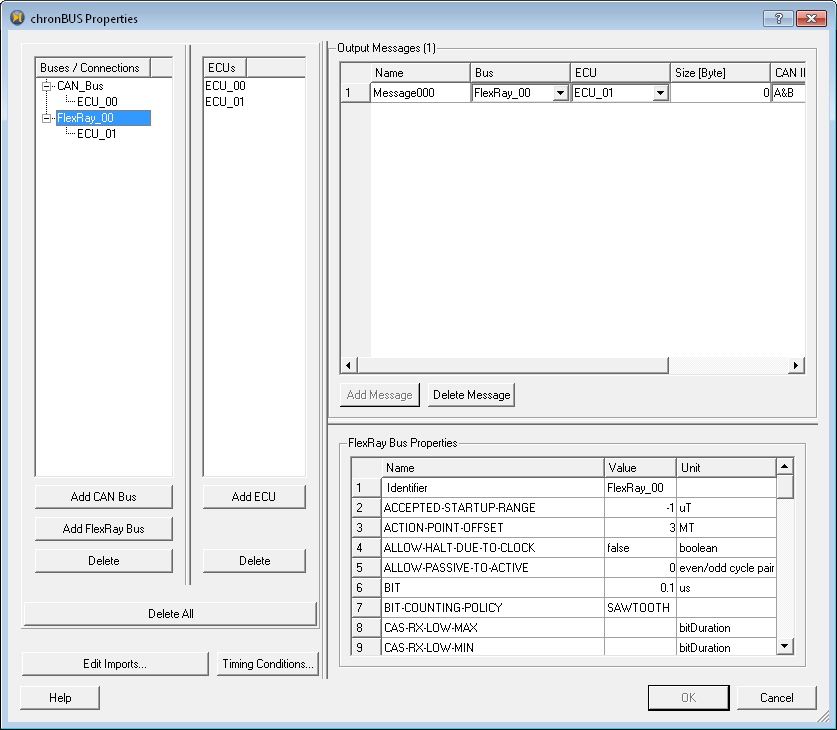
Figure 6.30: Rest Bus - Bus Properties #
CAN buses only have a single parameter: the bus speed. Parameters of a FlexRay bus are initialized with a default setting. The description of these parameters can be referenced in the FlexRay specification.
6.2.14.4.3 ECU Parameter #
In order to change ECU parameters, select an ECU from the ECU list. ECU properties are shown in the properties view at the bottom right of the dialog window.
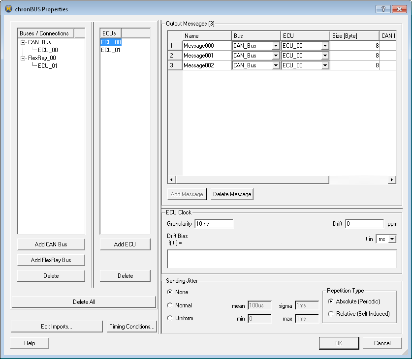
Figure 6.31: Rest Bus - ECU Properties #
Adjustable parameters are the ECU clock and message send jitter.
The send time of a message is calculated as follows:
tsend = (tscheduled + jitter + bias_function( tscheduled )) * drift #
6.2.14.4.4 Clock Parameters #
ECU clocks are configurable like processor clocks of the system model.
Granularity: the clock cycle of the discrete ECU clock
Drift: the ECU clock drift in ppm. A value of
-10 ppmfor an ECU clock with a granularity of10 nsslows the clock by1us(100 cycles) per second (compared to a simulated clock without drift).Drift Bias: Additionally to a constant drift factor a bias function may be applied. In the Drift Bias input field an arbitrary C expression as function of time variable
tmay be entered. A valid expression is t * 2.5 + 20. The expression may use constants and mathematical functions frommath.hof the C standard library. As an example the expression 1.0e-6 * sin( t * M_PI / 30 ) withtinswill yield a periodic drift bias with a cycle length of60s. The unit oftmay be chosen from the combo box.Sending Jitter: In real systems the send time of ECU messages may vary as a result of jitter of ECU internal processes like task scheduling or processing jitter. The jitter settings allow the statistical modeling of message send time variation as either uniform or normal distribution.
If Absolute Periodic is chosen as Repetition Type then the message send time will just be offset by a random jitter value. In case of Relative (Self-Induced), each message send jitter offset will be calculated relative to the send time jitter of the previous message.
6.2.14.4.5 Output-Messages #
The table Output Messages shows the messages of all connections selected in the bus connection tree view. Existing messages may be assigned to a bus ECU connection by using the clipboard.
Important:
Adding messages is only possible in context of a specific bus ECU connection. For that reason necessary to select a single ECU item in the connection tree in order to Add Messages.
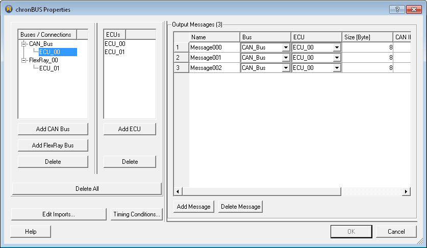
Figure 6.32: Output-Messages Table #
The size of message frames is adjustable. For CAN messages a unique CAN ID has to be assigned. For FlexRay messages a FlexRay channel has to be selected (A, B or both).
The following table lists the supported CAN message formats.
Table 6.1: Supported CAN Message Formats #
| Format | max. CAN ID | max. size [Byte] |
|---|---|---|
| Standard | 2047 | 8 |
| Extended | 536870911 | 8 |
| J1939 TP BAM | 536870911 | 1785 |
6.2.14.4.6 Message Timings #
The Message Timings of the selected message are shown in the property view.
Message sending is controlled by message timings. Message Timings are shown and edited in the property view below the Output Messages list. Activation of each Message Timing may be controlled with the check boxes of the enable column.
For CAN messages Cyclic Timings and Event Timings may be defined. For FlexRay messages either Absolute Scheduled Timings or Event Timings may be defined. Cyclic Timings may depend on Timing Conditions. Event Timings are triggered by Timing Conditions.
Time tolerances of message timings imported from FIBEX are not considered. For this purpose chronBUS uses message send jitter on ECU level.
6.2.14.4.6.1 Cyclic Timings #
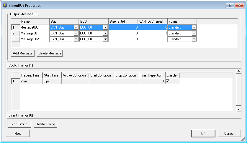
Figure 6.33: Cyclic Timings Table #
Cyclic Timings are relevant for CAN buses only.
Repeat Time is the cycle of a message
Start Time is the first send time
Active Condition is a comma separated list of system states („System Trigger“). At least one has to be set in order to activate a Timing.
Start Condition is a comma separated list of system states. At least one has to be set in order to start periodical sending.
Stop Condition is a comma separated list of system states, which stop periodical sending of the message.
Final Repetitions is the number of messages, which are sent after the stop condition occurs.
6.2.14.4.6.2 Event Timings #
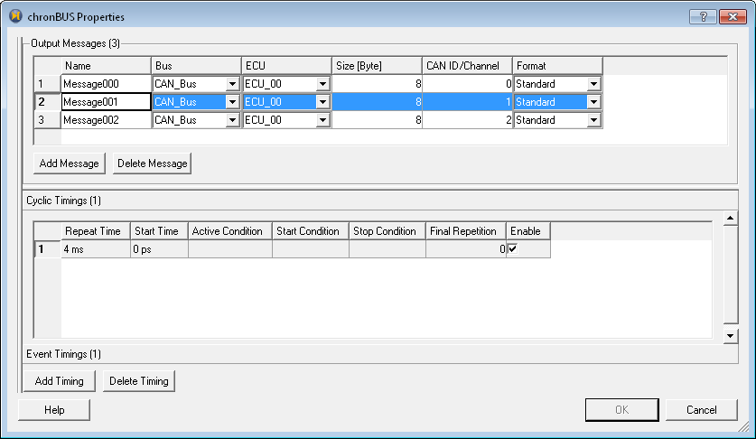
Figure 6.34: Event Timing-table #
De-bounce Time is the minimum time between two consecutive messages. In case of more send wishes up to one message will be buffered.
Active Condition is a comma separated list of system states („System-Trigger“). At least one has to be set in order to activate the timing.
Send Condition is a comma separated list of system states. At least one has to be set in order to trigger sending of the message.
Final Repetitions is the number of messages to be sent in case of the Active Condition.
6.2.14.4.6.3 Absolute-Scheduled Timings #
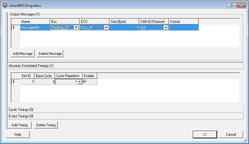
Figure 6.35: Absolute Scheduling Timing Table #
Absolute Scheduled Timings are relevant for FlexRay buses only.
Slot ID is the time slot of the message on the FlexRay bus.
Base Cycle is the cycle number of the message (
0 - 63.)Cycle Repetition: A value of e.g.
4specifies sending of every fourth cycle (1, 2, 4, ..., 64)
6.2.14.4.6.4 Timing Conditions #
Use the Timing Conditions... button to edit the list of all Timing Conditions used in the Message Timings. A Timing Condition represents a global system state. Each Timing Condition may be activated separately. Initially Timing Conditions are not activated.
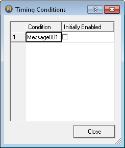
Figure 6.36: Timing Condition Dialog #
Alternatively the state of Timing Conditions during simulation may be controlled using a CSV stimulation file.
For this a stimulation scenario has to be defined with a CSV based Stimulation Generator as described in Section 6.7.2, “Defining a Stimulation Scenario”. For the stimulation source the parameters have to be chosen as follows:
Receiving Process: RestBus:StimPort
Stimulation Type: Read from CSV File
The CSV rows for controlling the Timing Conditions have the following structure :
<time in ns>, <time with unit>,
	      “<RestBusCondition>”, “<Condition>=0|1”
Each row defines the point in time of a Timing Condition state change.
In the following example the Timing Conditions actCond,
startCond and stopCond are activated after 1,
20 or 50 ms simulation time :
	      1000000, "1.000 ms", "<RestBusCondition>","actCond=1"
	      20000000,"20.000 ms","<RestBusCondition>","startCond=1"
	      50000000,"50.000 ms","<RestBusCondition>","stopCond=1"
6.2.14.5 Connect Rest Bus to System #
The buses of the rest bus may be used like buses of the system model. There is no functional difference for the simulation. The connection of buses of the rest bus with ECUs of the system to be simulated takes place in Module Architecture and is described in Section 6.2.7, “Peripheral Components”.
Rest bus buses are shown as ports in the system model in the rest bus element in Module Architecture. These bus ports are automatically connected to the rest bus.
6.2.14.6 Import of a System Description #
System descriptions for the rest bus may be imported from one or more external files. Currently the FIBEX and DBC formats are supported.
In case of FIBEX the name of all rest bus elements as well as
the unique IDs (e.g. of FIBEX tags <fx:CHANNEL>
and <fx:CHANNEL-REF> in case of buses)
of buses, ECUs and messages are imported into the rest bus model.
The names are imported as element identifiers and will appear in the lists and tables of
the rest bus editor dialog,
The unique IDs are shown in the rest bus editor as tooltip of the corresponding lists.
e.g. the ID of a bus is shown by moving the mouse over a bus item in
the bus connection tree.
Use the button to open the dialog for managing rest bus imports. Import files may be added or removed at any time. If an imported file is removed all its rest bus elements will be removed from the rest bus model.
A FIBEX file may be imported as follows:
Press and add the file
FIBEX.xml to the example project.
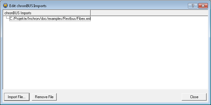
Figure 6.37: List of Imports #
Note:
If an imported file is removed all buses, ECUs, messages and message timings defined by it will be removed from the rest bus model.
After closing the dialog with the button the rest bus model contains all elements added by the import (s. Figure 6.38, “Rest Bus Model”). In this case the ECU list shows nine additional ECUs.
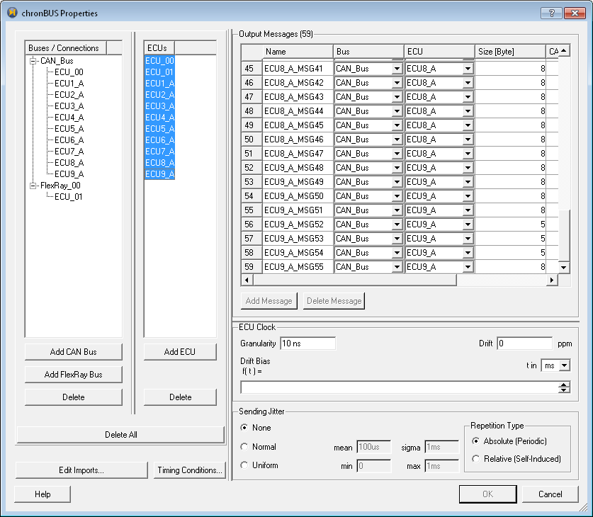
Figure 6.38: Rest Bus Model #
Usually a bus of a FIBEX description results in a new bus in the rest bus model.
However if, like in this example, the ID of the CAN bus from the FIBEX system description conflicts with the Bus-ID of the Bus CAN_BUS already existing in the rest bus model. Thus no new bus is created and the imported ECUs are connected to the existing bus.
6.2.14.7 Rest Bus in Diagrams #
The effect of the rest bus on the simulated system may be observed in the chronSIM state and load diagrams. Latency Histograms allow to analyze latencies of bus messages sent by ECUs of the system model. A more detailed description of these and other chronSIM diagrams can be found in Section 7.7, “Visualization”.
6.2.14.7.1 State Diagram #
The State Diagram shows a timeline of all sent messages separately for each bus. CAN messages are designated with their CAN ID, FlexRay messages with their Slot ID. For CAN buses the color of messages shown indicate the sending ECU of the system model. Messages from rest bus ECUs are shown gray by default which may be changed with → .
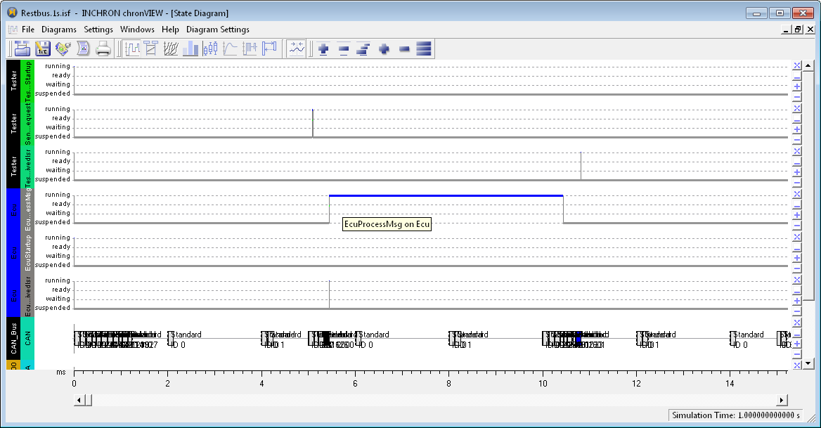
Figure 6.39: State Diagram #
6.2.14.7.2 Load Diagram #
The Load Diagram shows the load of processors, ECUs and buses of the system model over time.
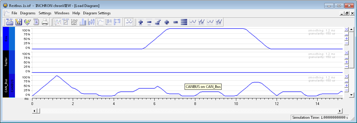
Figure 6.40: Load Diagram #
6.2.14.7.3 Latency Histograms #
A histogram allows the analysis of latency distributions. The following figures shows the latencies between request messages sent by the tester and responses by the ECU. For this, the histogram has to evaluate simulations events of the CAN controllers of the system model. The histograms below show the latency distribution of the FrameEnd events of both ECUs CAN controllers for two simulations (first without and second with rest bus workload). A FrameEnd signal on a receiving controller represents the point in time on which a CAN message was received.
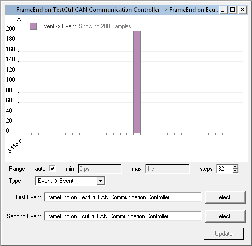
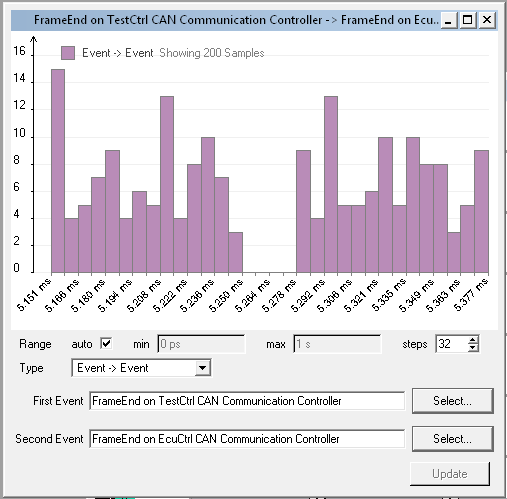
Figure 6.41: Histogram: Latencies without and with Rest Bus #
The first histogram shows the resulting latency for the system being simulated without rest bus workload.
For task EcuProcessMsg the response latency
has a fixed value of 5 ms mainly due to message processing time.
The second histogram illustrates the spreading of latency of the same
system when simulating with rest bus workload.
The response latency for task EcuProcessMsg now spreads
in a range from 5.14 ms to 5.37 ms.
The increase in latency is the consequence of delays caused by
rest bus messages with low CAN ID (and thus high priority).
After importing the FIBEX system description Fibex.xml
the simulation will show an even higher bus workload which will lead to considerably increased latencies.
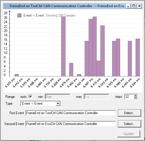
Figure 6.42: Histogram: Latencies After FIBEX Import #
6.3 Module Architecture #
For the following explanations, please load a project with peripheral hardware components
like e.g.
sync2flexray.ipr from subdirectory
sync2flexray.
Resize the project window to a size suiting you best and select the architecture module.
6.3.1 Concept of Module Architecture #
The purpose of the module „Architecture“ is the editing of hardware components and port connections of the system model. Connections are made between
peripheral components: external components like UART, memory, buses and bus controllers, D/A or A/D converters
buses and controllers of an optional chronBUS rest bus model
A tree view shows all hardware components of the system model. Components are added and removed in the same way as in module System as described in Section 6.2.7, “Peripheral Components”.
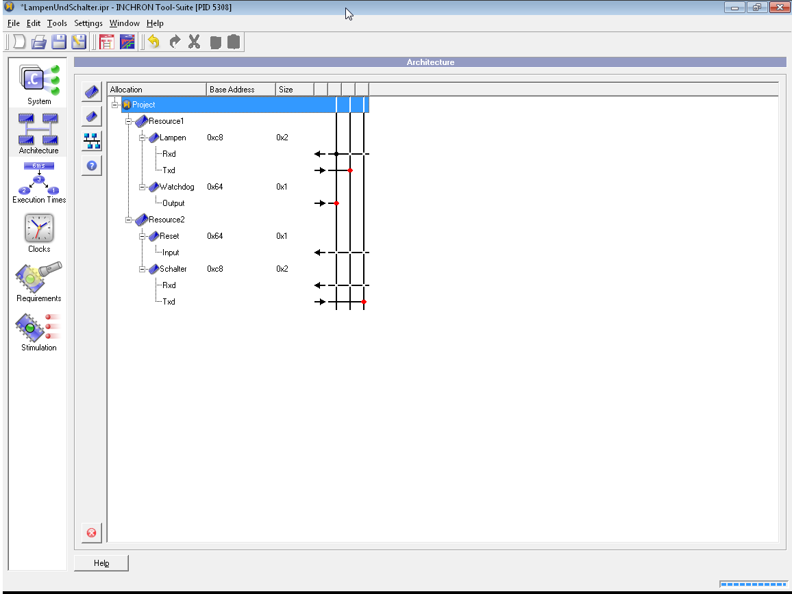
Figure 6.43: Architecture View with Port Connection Matrix #
6.3.2 Peripheral Connections #
Peripherals and buses for being connected have predefined ports of certain types. Ports have either input/output characteristics, facilitating the transfer of numerical data or are interrupt ports (named IRQ) for activation of an interrupt handler.
For establishing a connection between two i/o ports, two connection dots on a vertical line in the connection matrix are required.
Important:
The horizontal line of each output port in the connection matrix automatically shows a fixed red dot on the crossing of a corresponding vertical line. The respective vertical line is reserved for connecting input ports to the output port.
A connection point is set or removed by a crossing point of a vertical and a horizontal line in the connection matrix.
Note:
The connection of incompatible ports e.g. two output ports is not possible.
6.4 Module Execution Time #
For the following explanations please load the example project simple.ipr
from the functionnesting folder.
6.4.1 Concept of Module Execution Time #
The chronSIM simulation requires detailed information about the execution times of the source code on the target platform. The module Execution Time allows the analysis and manual specification of static execution times each code block consumes on the target. With the Tool-Suite's chronEST option it is possible to automatically determine the static execution times of the source code on the selected target. Without the chronEST option you can still enter execution times of basic blocks manually.
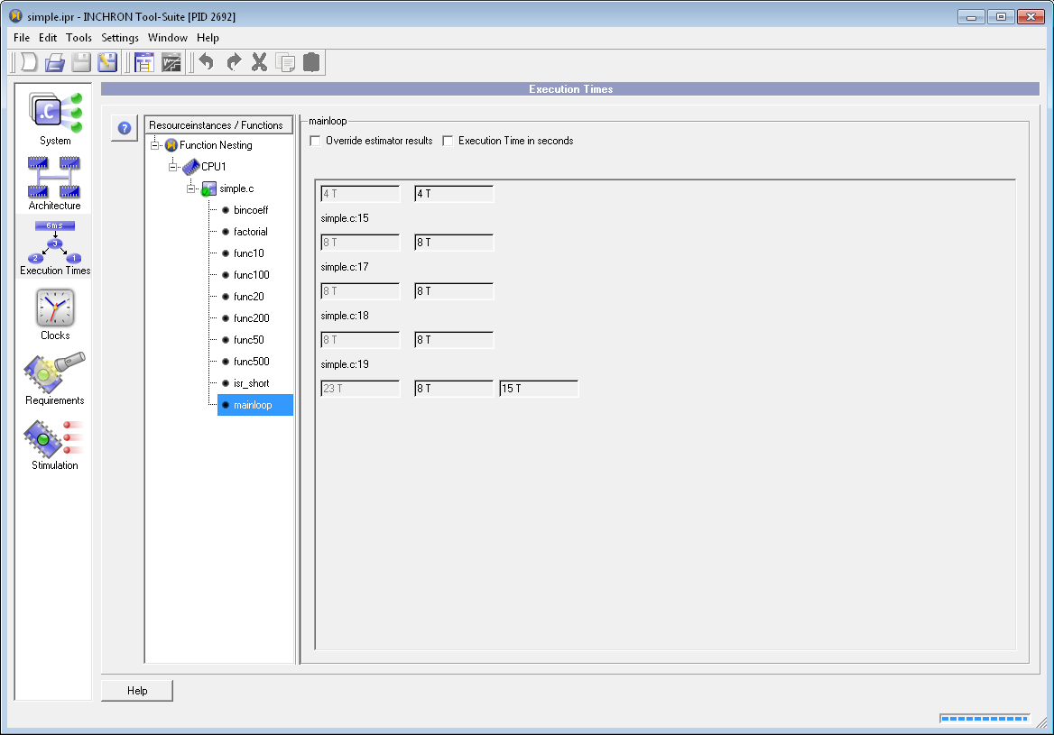
Figure 6.44: Module Execution Time #
6.4.2 Execution Times View #
Load the
dect.iprexample project.Select the module Execution Time.
In the tree view select a clock item.
The right area of the window displays the execution times of basic blocks which were automatically determined by chronEST as shown in the screenshot below.
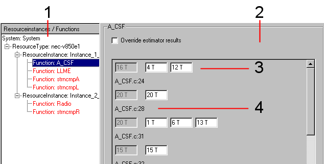
Figure 6.45: Module Execution Time #
The numbered elements denote
List of the execution times of all parts of the function
16T: field displaying the cumulative number of clock cycles of this function or code block. This is followed by fields showing clock cycles of the code blocks which were summed up.Corresponding source code file name and line number, e.g.
A_CSF.c:24
To give a better understanding the relation between the execution times and the source code is illustrated in the following two figures. The first shows a control flow graph (CFG) of a function fragment and how each graph node relates to a corresponding basic code block in the C source code.
The second figure shows how the assigned execution times in the Tool-Suite GUI correspond to nodes in the flow graph.
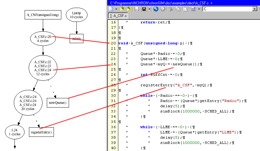
Figure 6.46: Control Flow Graph Nodes and Corresponding Source Code Basic Blocks #
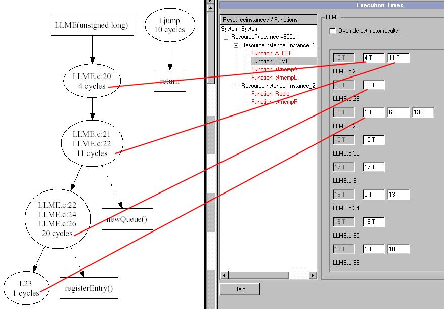
Figure 6.47: Control Flow Graph Nodes and corresponding Execution Times #
6.4.3 Automatic Estimation with chronEST #
chronEST automatically determines the execution times of your source code considering specific timings of the chosen processor model (see Section 6.2.6.2, “Processor Properties”). The estimated execution times depend on the selected optimization options of the target compiler. The automatically determined execution times of your source code can be manually overridden for testing legacy as part of the system architecture or checking partially implemented routines against their specification. Before starting a simulation you may manually modify the automatically determined execution times.
6.4.4 Manually Overriding Estimations #
The manual specification of execution times is typically employed during the early phase of a development project as the final source code of the intended software is not yet available.
That way the overall system architecture can be designed and checked for general conformity with its specification. The execution times can be entered manually on a function and basic block granularity.
In order to manually specify execution times or to override execution times evaluated by chronEST do the following:
Select a function in the tree view.
The right area of the window now displays the execution times of this function which were automatically determined by chronEST
Check the option in the right window area.
the corresponding execution time input field.
Enter the number of clock cycles xy T to specify the intended simulation time of the corresponding function.
Repeat steps 1 to 5 for all source code functions whose execution times you wish to override.
Finish your modifications by clicking Apply or discard all modifications by clicking Reset.
6.4.5 Control Flow Graph #
INCHRON Tool-Suite is able to display control flow graphs of all your source code’s functions. Obey the following steps to view the control flow graphs of a function:
the context menu with a on the function of interest In the system.
Select View Control Flow Graph from the context menu.
The control flow graph will be processed and then displayed in an external viewer.
You can export the control flow graph to a file using the save to file functionality of your PDF viewer.
6.5 Module Clocks #
For the following explanations please load the example project
sync2flexray\sync2flexray.ipr.
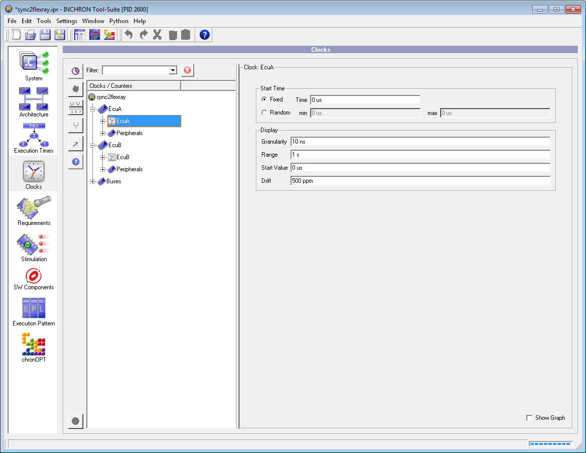
Figure 6.48: Module Clocks #
6.5.1 Concept of Module Clocks #
Microcontroller components need a clock signal as a time base for their operation. The purpose of module Clocks is to configure the parameters of the simulated systems hardware clocks. These clocks are also the source for stimuli scenarios defined in module Stimulation.
6.5.2 Implicit Processor Clock #
The predefined microprocessor targets contain a hardware clock. For each processor instance added in module System the corresponding clock will also appear in module Clocks.
6.5.2.1 Start Time of a Clock #
The start time of the implicit processor clock also defines the start time of this processor and its peripherals.
Similar to a stimulation generator the startup time can be configured as either fixed with a predefined delay, or random with a uniform distribution between a minimum time and a maximum time. The default is a fixed startup time with a defined delay of zero (0 seconds).
6.5.2.2 Effects of a Start Time #
The configured start time of a clock influences or delays the following model elements:
Processor startup
Start of active-at-boot processes
Activations of processes are dropped if the start time has not yet expired
Start of TDMA scheduling
Peripheral startup, e.g. FlexRay cyclestart or Ethernet handshake
Stimulations which reference this clock
6.5.3 Parameters of a Clock #
Besides the start time (which is mainly interpreted for microprocessors) a clock has the following parameters:
Granularity: The length of a clock tick, i.e. the period, which is the inverse of the frequency.
Range: This is the range which the clock can display before it overflows and starts again at 0s.
Start Value: The displayed value of the clock when it starts.
Drift: The drift of a clock is specified in ppm (parts per million). It specifies the deviation of this clock from the global ideal time. A clock with a negative drift will run faster.
6.6 Module Requirements #
- 6.6.1 Concept of Module Requirements
- 6.6.2 Requirement Types
- 6.6.3 Process Net Execution Time Requirement
- 6.6.4 Event Net Execution Time Requirement
- 6.6.5 Net Slack Time Requirement
- 6.6.6 Response Time Requirement
- 6.6.7 Event Timing Requirement
- 6.6.8 Illegal Event Requirement
- 6.6.9 RTOS Failure Requirement
- 6.6.10 Event Periodicity Requirement
- 6.6.11 Load Requirement
- 6.6.12 Event Chain Timing Requirement
- 6.6.13 Import and Export of Requirements
For the following explanations please load the example project sync2flexray.ipr.
Select the module Requirements as shown below.
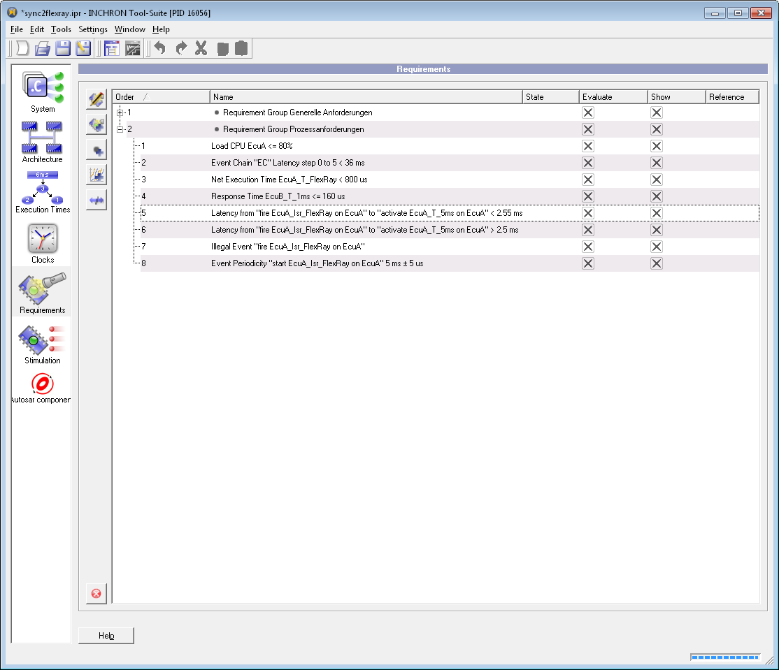
Figure 6.49: Module Requirements #
6.6.1 Concept of Module Requirements #
The Module Requirements is an editor for real-time requirements. Real-time requirements are dynamically evaluated during simulation of the project (see Section 7.6, “Real-Time Requirements”) and resulting evaluations are shown in simulation diagrams (see Section 7.7, “Visualization”). The requirement view of the simulation window shows a summary of the requirements evaluations and may be exported in different formats (see Section 7.10, “Reporting”).
The Module Requirements is used for the specification of the project's real-time requirements.
The supported types of real-time requirements usually evaluate the violation of a certain limit, which is a timing criterion in case of timing requirements (e.g. response time of a process or more general the latency of two specified events), a load percentage for CPU or communication resources or a counter. The function nesting requirement is an example of a functional requirement.
Requirements may be added, removed, edited and structured hierarchically:
Use the corresponding buttons on the left for adding a requirement or a requirement group.
Double clicking an existing requirement will invoke the dialog for editing its properties.
Requirements may be rearranged by drag and drop.
Existing requirements may be edited by double click and rearranged by drag and drop.
The menu offers options for import or export of requirements. In order to link a requirement to an external requirement management system like DOORS®, each real-time requirement may have an external reference URL which is shown in the Reference column of the requirement tree view.
The simulation mode has its own requirement editor (see Section 7.6, “Real-Time Requirements”), which not only allows for editing of requirements but also visualizes requirement evaluation results during chronSIM simulation. [3].
Individual requirements or whole requirements groups may be excluded from evaluation using the checkboxes in the Evaluate column of the requirement tree view. Visualization of evaluations in diagrams may be toggled using checkboxes in the Show column.
6.6.2 Requirement Types #
Currently the following types of functional and timing requirements are available:
- Call Nesting
Limit the function call depth (stack).
- Recursion
Limit for function recursion.
- RTOS Failures
Failed in case of RTOS Failures.
- Requirement Group
Container element for hierarchical structuring of requirements.
- Process Net Execution Time
-
A timing requirement for validation of process or ISR net execution time.
- Event Net Execution Time
-
Net Execution Time between two arbitrary events of a single process. I.e. execution of (non-recursive) functions or runnables are also covered by this.
- Net Slack Time
Remaining capacity for a process (or ISR) terminating before its deadline.
- Response Time
Response time (i.e. time from activation to termination) of a process or ISR.
- Event Timing
Time between two arbitrary events (e.g. ISR or process activation, start or termination, function entry or user defined event).
- Illegal Event
An Illegal Event counts as violated every time if its event parameter occurs during simulation.
- Event Periodicity
An Event Periodicity requirement evaluates the distance of consecutive periodic events to be in specified limits.
- Load
Load on CPU or bus resources.
- Event Chain
Time between steps of an Event Chain.
- Event Chain Break Off
Unterminated Event Chain.
- Event Chain Multiple Processing
Event Chain with multiple occurrence of same step.
- Event Chain Join
Join of forked Event Chain.
The requirement types Call Nesting, Recursion and RTOS Failure are functional requirements. The requirements Call Nesting and Recursion refer to a function call and evaluate as Failure if the defined limit for a specified function is violated by entering the function. An RTOS Failure requirement evaluates as violated, as soon as a RTOS Failure occurs (e.g violation of task activation limit).
Timing Requirements#
The requirement types Process Net Execution Time, Event Net Execution Time, Response Time and Event Timing are timing requirements. For evaluation of a timing requirement two consecutive events defining a time interval are checked against a given time limit. This allows e.g. the verification of execution time budgets of processes and functions.
6.6.2.1 Evaluation Verdicts #
Beside of the usual evaluation verdicts successful and failed many requirement types like timing requirements, load requirement allow for a third evaluation type (verdict) called critical. For this a certain range between successful and failed evaluation has to be defined. This is done editing a requirement and specifying a Prewarn Margin, which is always relative to the requirement's limit value. The margin for the critical limit may be specified either in unit of the limit or as percentage of the limit by checking the relative option.
6.6.3 Process Net Execution Time Requirement #
This timing requirement evaluates net execution times of a process or ISR. I.e. the evaluated times exclude time intervals where the process under investigation is preempted by higher priority tasks or ISRs.
Mandatory parameters are a target process or function and a maximum execution time. To facililtate critical evaluations an optional prewarn margin may be specified.

Figure 6.50: Process Net Execution Time Requirement #
6.6.4 Event Net Execution Time Requirement #
This timing requirement evaluates net execution times between consecutive occurence of two specified events of a process (or ISR). Like with the Process Net Execution Time Requirement evaluated times exclude time intervals where the process under investigation is preempted by higher priority tasks or ISRs.
Mandatory parameters are a start and an end event of a process (or ISR). Additionally, a process has to be given if it is not implicit (which is the case if two function events are given, because it is not known in advance which process will execute it).
As with other requirement types, to facililtate critical evaluations an optional prewarn margin may be specified.
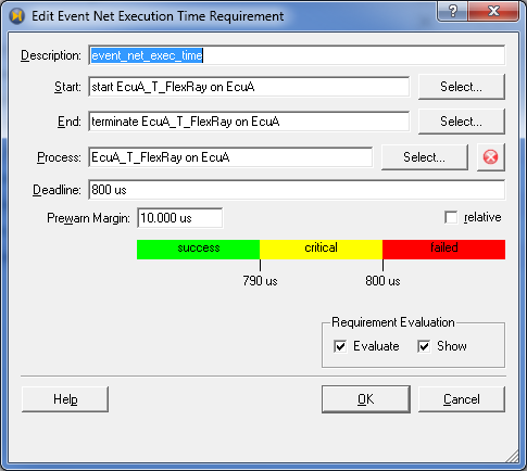
Figure 6.51: Event Net Execution Time Requirement #
6.6.5 Net Slack Time Requirement #
A net slack time timing requirement checks a constraint for the time between termination and the deadline of a process (or ISR), which is a measure for remaining capacity.
Note:
The net slack time for a process execution ending before its deadline is defined as the sum of remaining time in the time interval from process termination until the end of its deadline, where no higher priority process (or ISR) is running.
Hence the definition of a net slack time requirement requires the definition of a process deadline. In the dialog of the net slack time requirement this can be specified either
directly,by giving an explicit duration (starting from process activation) or alternatively
indirectly by defining an arbitrary simulation event. The deadline in that case will be calculated as the time interval from process start to the next occurance of the given event.
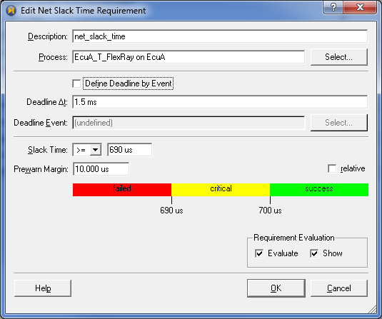
Figure 6.52: Net Slack Time Requirement #
Tip:
For a worst case analysis of remaining capacities using chronVAL, see Section 8.3, “Example of Analyzing a Distributed System” and Figure 8.12, “Remaining Capacity as Interval Diagram”.
6.6.6 Response Time Requirement #
A response time timing requirement checks the time between activation and termination of a process. Mandatory parameters are a target process and the maximum response time [4].
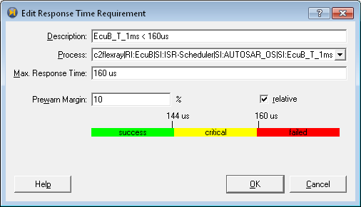
Figure 6.53: Response Time Requirement #
In contrast to the net execution time requirement measured response times include process preemptions by higher priority processes or ISRs.
Tip:
For the case of of OSEK extended tasks the response time requirement is not suited to evaluate meaningful task response times since extended tasks will run unterminated and thus have no terminate events during simulation. However, in this case you may evaluate response times beween the tasks Block and Restart events using the more general Event Timing Requirement.
6.6.7 Event Timing Requirement #
The Event Timing requirement facilitates evaluation of more generic latencies between event occurencies. Its definition requires three events: a trigger event, a start event and an end event.
Each time a trigger event occurs, the time difference between the last start event and the last end event is evaluated. Trigger and end event may be identical (recommended).
For each of these three events any simulation event from your system model may be chosen. The requirement's events are specifed using the Object Selection Dialog described in the next subsection.
The relation between specified time limit and the simulated time may be specified with the operators <, <=, > or >=.
The start, stop and trigger event may be chosen from the following events of the system model:
The activate, start and terminate events of the model's processes or fire, start and stop events of the ISRs
The entry and exit events of functions defined in the model's source code.
The events resulting from
EVENT()andEVENT1()instrumentation in the model's source code.
Tip:
The Event Timing requirement is not suited for evaluation of individual data flow instances (see Section 6.2.13, “Event Chains”). For this purpose the dedicated Event Chain requirement has to be used.
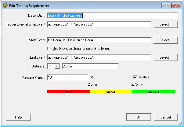
Figure 6.54: Event Timing Requirement #
The parametrization of the Event Timing Requirement requires the selection of simulation events. By clicking an event (or the right to it) the Object Selection Dialog will be shown.
6.6.7.1 Object Selection Dialog #
This dialog presents the appropriate entities from your project's system tree. Depending on the context, these may be, for example, simulation events, peripheral ports or the functions all translation units of the current CPU resource as leave nodes.
The following image exemplifies an Object Selection Dialog showing all implicit and explicit (instrumented) events (see Section 7.2.5, “Simulation Events”). I.e. process events appear as children of processes and function and explicit events as children of translation units.
Because the number of events may be huge in a project, the dialog offers a convenient way of filtering elements by name via the Filter input field:
For flexible filtering, the expression entered may be a name substring or a regular expression
The filter expression does not act on names of the leave nodes alone, but on the element's whole tree path instead. The tree path is shown as tooltip and contains type prefixes like e.g.
P:for processes
Thus to filter function events of function myFunction in file file1.c
on resource MainProcessor
you may enter the filter expression MainPr.*myFun
[5]
and for showing any process start event on resource MainProcessor
just use the expression MainPr.*start.
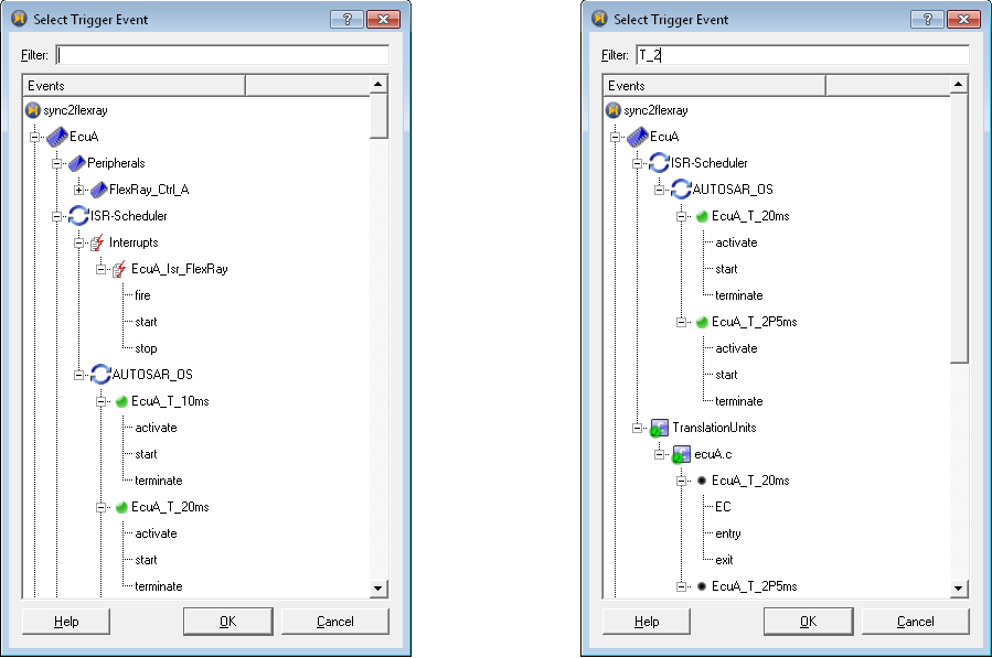
Figure 6.55: Object Selection Dialog - unfiltered versus filtered event tree #
6.6.8 Illegal Event Requirement #
This requirement defines an ordered sequence of arbitrary implicit or explicit simulation events (see Section 7.2.5, “Simulation Events”). Each occurrence of this sequence will be evaluated as a requirement violation.
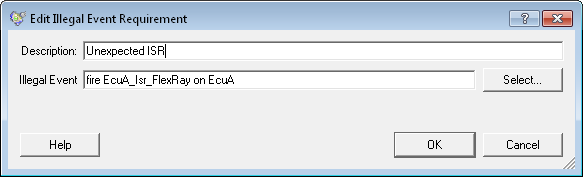
Figure 6.56: Illegal Event Requirement #
6.6.9 RTOS Failure Requirement #
A RTOS Failure requirement can be used to detect RTOS failures of selected type for selected tasks. The types can be selected by checking one or more RTOS failure types in the 'RTOS Failure Types' list.
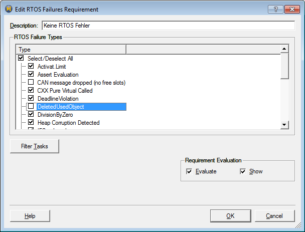
Figure 6.57: RTOS Failure Requirement - type selection #
When the button is pressed a dialog opens to select specific tasks for which RTOS failures shall be detected.
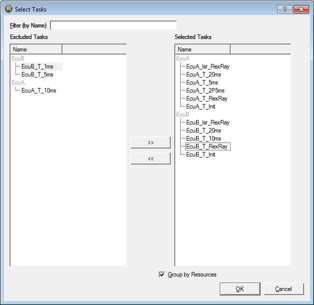
Figure 6.58: RTOS Failure Requirement - task selection #
6.6.10 Event Periodicity Requirement #
The Event Periodicity requirement checks the distance between successive occurrences of an arbitrary implicit or explicit event (see Section 7.2.5, “Simulation Events”) to be in a specified time range.
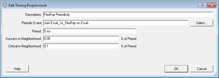
Figure 6.59: Event Periodicity Requirement #
6.6.11 Load Requirement #
Load requirements may be defined on CPU or bus resources
Using a load requirement you may monitor a CPU or bus resource for
violations of a given load limit in a given (sliding) time window.
The evaluated load may also be interpreted as an equivalent of CPU power consumption.
Load requirements for FlexRay buses evaluate the dynamical segment only.
[6].
The following images relate to the predefined load requirement
of the sync2flexray.ipr example project
and illustrate resulting requirement evaluations.
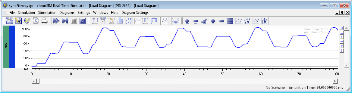
Figure 6.60: Load Diagram #
With the chosen smoothing value of 5 ms
the resulting load shows periodic peaks every 10 ms
with alternating peak values of about 80% and 100%.
The Averaging Interval equals the smoothing parameter of the load diagram and evaluates as the product of number of steps and step size (granularity) as given by the input field on the right.
Note:
The Averaging Interval is not a parameter of the requirement evaluation itself but only of the preceding estimation of load values (see Section A.2, “Load Calculation” for details on load calculation).
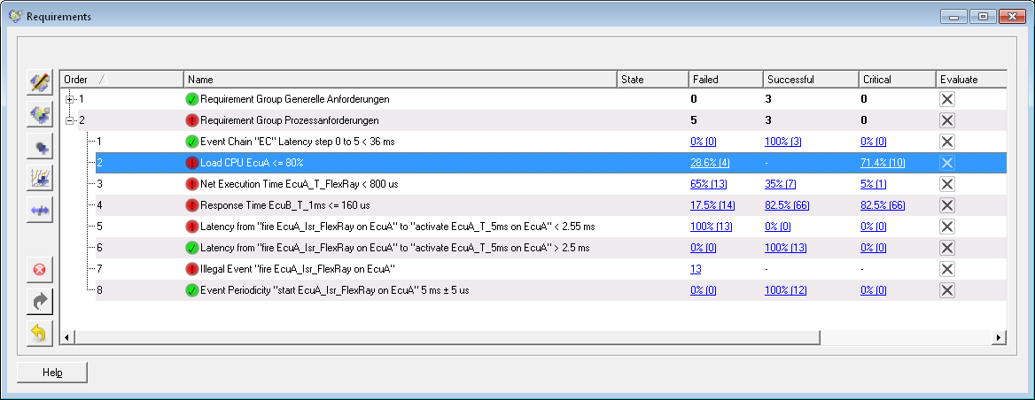
Figure 6.61: Load Requirement #
The predefined load requirement of the example has a load limit of 80%.
Due to the prewarn margin
of 10% the limit for critical evaluations is at 70%.
This results in the load requirement evaluating as failed every 20ms
and as critical every 10ms.
Tip:
For the load diagram in order to show equivalent load values as evaluated for a load requirement, the diagram's smoothing value should equal the requirement's Averaging Interval (and the granularity should resemble the requirement granularity value).
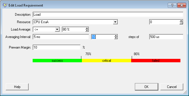
Figure 6.62: Requirements Overview #
The requirement settings shown above lead to four requirement failures
and eight critical evaluations in the first 80ms of simulation.
If the Averaging Interval is increased by either
raising the granularity interval or the number of averaging steps the load
requirement will no longer evaluate failures:
With values of the Averaging Interval above 10ms the
mean load will always be below the limit of 80%.
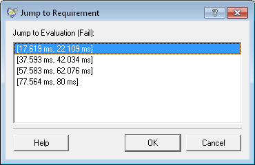
Figure 6.63: Load Requirement Evaluations #
6.6.12 Event Chain Timing Requirement #
An Event Chain Timing Requirement checks the time between two steps of an event chain. In order to use Event Chain requirements the model's source code has to be instrumented (see Section 6.2.13, “Event Chains”). An Event Chain Timing Requirement has the following mandatory parameters:
An event chain name
the steps Step A and Step B
the timing criterion to be checked
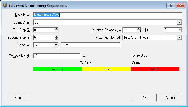
Figure 6.64: Event Chain Timing Requirement #
In case chain instances during simulation do not statically start with a specific step, you may specify the special value first in instance for Step A to always match the first occurring step of each instance. In the same way you may specify special value last in instance for Step B to always match the last occurring step of each chain instance.
The following parameters are optional:
In case the steps do refer to different instantiations of the Event Chain a Instance Relation may be specified as a linear relation between the instantiations of the steps Step A and Step B.
In case duplicates of Step A or Step B may occur within a single Event Chain instantiation an appropriate Matching Method may be chosen. Using the default setting First A with First B, the first Step A and Step B of an instantiation will be evaluated.
6.6.13 Import and Export of Requirements #
Real-time requirements of an INCHRON project are usually stored as part of the project file.
Furthermore a project's real-time requirements can be exported to
or imported from the INCHRON specific IRQ format
via the menu of the Tool-Suite main application window,
which facilitates processing of additional sets of requirements
with chronVIEW
or the chronSIM Batch simulation.
.
Also, for purpose of interoperability a set of requirements can be imported from or exported to a DOORS® requirement management system as described as part of Chapter 11, Integration with IBM Rational Software. The INCHRON Tool-Suite stores the references while allowing to refine the textual DOORS requirements with technical real-time requirements which can be evaluated automatically. See Section 11.2.2, “Importing Requirements from DOORS” on how to do this.
6.7 Module Stimulation #
For better understanding please load the example project
dect_scenario.ipr from subdirectory dect.
6.7.1 Concept of Module Stimulation #
The stimulation of the simulation model is controlled by parametrized generators. A stimuli generator generates a periodic or aperiodic pattern of stimulation events with optional random variation. Multiple stimuli generators may be combined in a stimulation scenario in order to define ore complex stimulation patterns. In case of multiple stimulation scenarios only one may be selected as the active scenario to affect the simulation. While a generator can only be used in a single scenario a scenario itself can be reused in one or more Composite Scenarios. Such composite scenarios reference one or more (normal) scenarios with all of them being active at the same time (see Section 6.7.3, “Composite Scenario”).
A stimulation generator may target a process (or ISR), a peripheral component or a runnable entity. You can superimpose your stimulation with additional disturbances like drift, EMC interferences or irritations caused by harmonics and build feedback loops by connecting output signals to inputs.
All generators in a scenario are starting at relative time t=0s if the scenario is used in the simulation or validation. A scenario can also have a burst filter defined which limits the number of events in a specified time period. See Section 6.7.2.7, “Limiting Stimulations with a Burst Filter” for details.
Stimulations can be loaded and included into your simulation from external files (CSV files) as well.
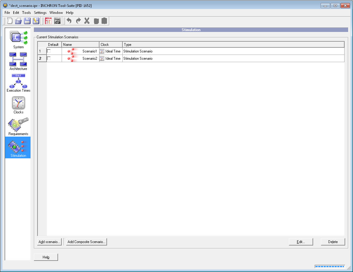
Figure 6.65: Module Stimulation #
Apart from that the environment can be modeled and included as simulated processes using C source code, thus enabling you to model complex feedback control loops.
6.7.2 Defining a Stimulation Scenario #
- 6.7.2.1 Stimulation Scenario Parameters
- 6.7.2.2 Stimulation Generators
- 6.7.2.3 Selecting the Target
- 6.7.2.4 Configuring the Stimulation Generator
- 6.7.2.5 Stimulation Parameters - Disturbance
- 6.7.2.6 Stimulation Parameters - Drift
- 6.7.2.7 Limiting Stimulations with a Burst Filter
- 6.7.2.8 Stimulation Preview
In order to use stimulation for your simulation model it has to provide appropriate input targets.
For the stimulation of your simulated target one or a number more alternative stimulation scenarios have to be defined. A scenario consists of one or more stimulation sources with each source generating a specific stimuli pattern for one input. This composition enables you to specify almost arbitrary complex stimulations for stimulating your simulated target system.
To apply a stimulation scenario to a simulation run it has to be explicitly activated. This activation is done after the simulation model was created or by marking it as Default scenario in the project window’s stimulation module. You may also manually apply additional single stimulations to a running simulation at any time.
6.7.2.1 Stimulation Scenario Parameters #
6.7.2.2 Stimulation Generators #
For each stimulation source of a stimulation scenario a stimuli generator has to be defined. A stimulation source is characterized by
the type of stimulation
target (receiving) process, busmessage or environment variable
starting time of the stimulation
repetition rate
variation
disturbance
The scenarios and their associated stimulation sources are part of the simulation model and are saved to the project file (IPR).
Obey the following steps to create a stimulation scenario:
Load the example project
isr\bursty.ipr.Select the module Stimulation.
Press or on an existing scenario.
The Add Stimulation Scenario window becomes visible as shown in the screenshot below. Adjust the size of this window according to your preferences.
The dialog window for defining the stimuli sources for a scenario is divided into two parts. The upper part shows a preview of your already defined stimulation sources. The window part below shows the parameters of the specified stimulation sources.
Enter a unique identifier for your stimulation into the Scenario Name input field.
Continue by selecting the intended time base from the drop down menu Base Clock with your left mouse button. All time bases from the Clocks module and the standard time base Ideal Time can be selected.
Press or into the still empty input field Current Scenario to configure a new stimulation source.
The Stimulation Parameters dialog for the parametrization of the stimulation source appears (see the following section).
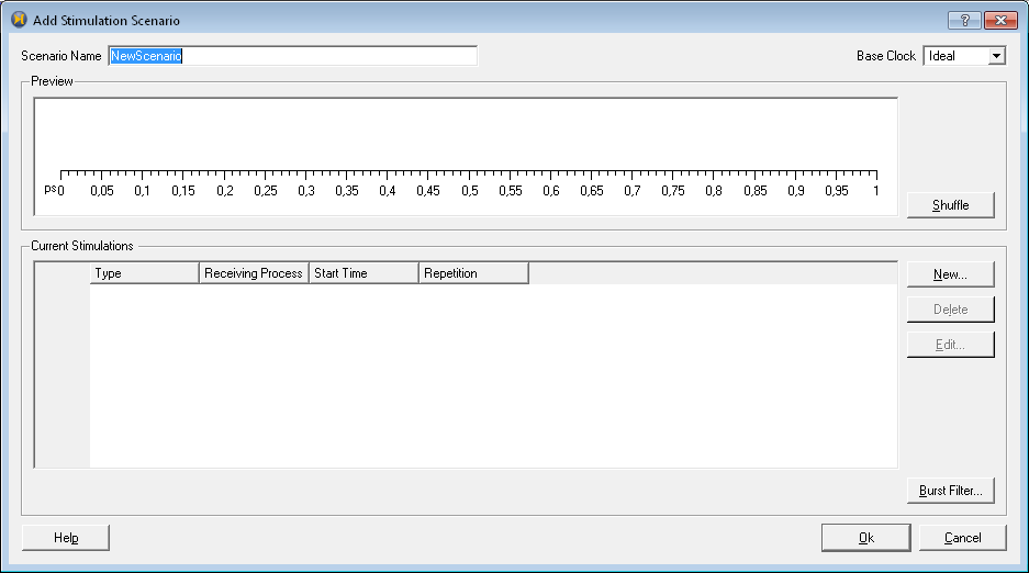
Figure 6.66: Add Stimulation Scenario Dialog #
6.7.2.3 Selecting the Target #
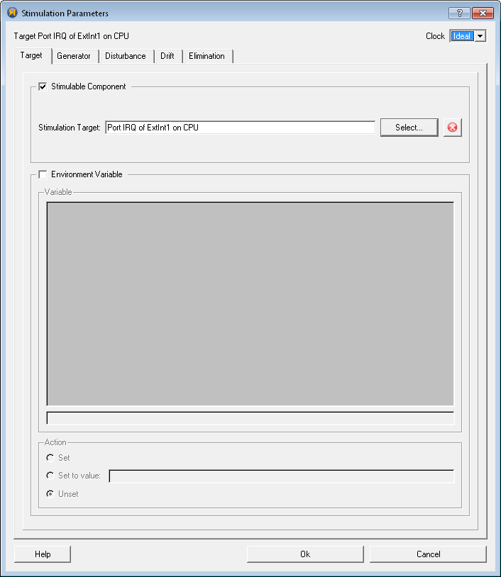
Figure 6.67: Tab Target #
On the Target tab the target of the stimulation generator is configured. In the upper half are the elements of the project selectable (processes, interrupts, bus messages). The lower half manages environment variables (see Section 7.4, “Environment Variables”) which can be set or unset from scenarios.
To change a stimulation target check the Stimulable Component option and click the current target or the . An object selection dialog opens. Select the intended item and confirm with .
To stimulate an environment variable check the Environment Variable option. New environment variables are entered in the line edit below the list. As action either Set (a defined but empty variable), Set to value, or Unset (the variable is deleted) can be selected. Defined variables from other stimulation generators are shown in the list and can be selected easily.
The selected operation changes the variables value or existence when the stimulation generator creates an event. The variable keeps its value until the next change. To set a variable VAR between 1s and 2s therefor two generators are needed: One for setting VAR at 1s and one for unsetting it at 2s.
6.7.2.4 Configuring the Stimulation Generator #
To edit the type and the parameters of a stimulation generator select the Generator tab.
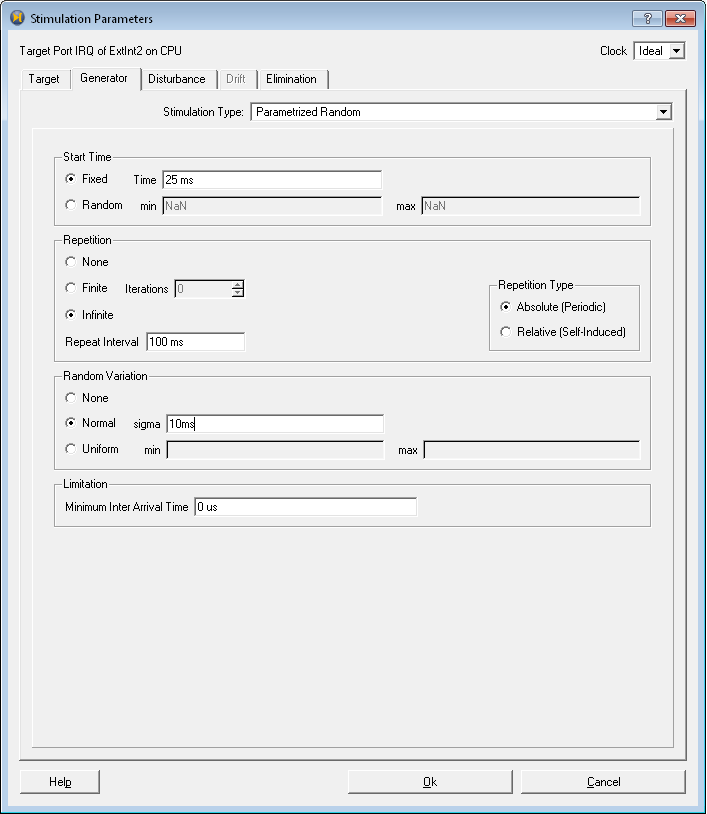
Figure 6.68: Tab Generator #
INCHRON supports the following Stimulation Types:
Parametrized Random
Burst Pattern
Read from CSV File and
Induced
List Based
Induced List Based
Time Units. The configuration of a stimulation generator requires the specification of timing parameters. INCHRON Tool-Suite supports the following time units:
s for seconds
ms for milliseconds
us for microseconds
ns for nanoseconds
ps for picoseconds
C or T for cycles of the microprocessor's clock (see Section 6.2.6.2, “Processor Properties” or Section 6.5.2, “Implicit Processor Clock”).
6.7.2.4.1 Parametrized Random #
This Stimulation Type allows for flexible configuration of cyclic and/or random stimuli generation.
Start Time denotes the start of the stimulation. For the stimulation of your simulation model the following time units are available: The start time of the stimulation may be specified
The Repetition of a single stimulation may be
switched off by selecting None or
Absolute (periodic) or
Relative (self Induced).
with the number of repetitions being
For periodic stimulation you may specify a superimposed Random Variation:
Normal variation around the given Repeat Interval with variation Sigma.
Uniform variation between Min and Max.
The following diagrams illustrate the stimuli generation. The colored arrows represent generated stimuli. The gray curves in the latter diagrams show the probablity distribution of random variation.
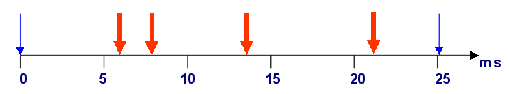
Figure 6.69: Stimulation from Random Generators #
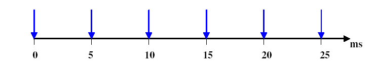
Figure 6.70: Absolute Periodic Stimulation #
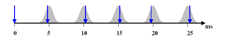
Figure 6.71: Absolute periodic Stimulation With Normal Distribution #
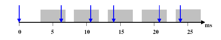
Figure 6.72: Absolute Periodic Stimulation With Uniform Distribution #
6.7.2.4.2 Read from CSV File #
This Stimulation Type allows for importing of stimuli e.g. from field tests. Importing stimulation data from a CSV file is done as follows:
Select Read from CSV File from the drop-down menu.
Select the CSV file by ing the icon on the right.
Use the file open dialog to select the desired CSV file.
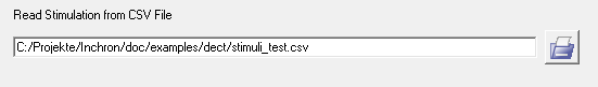
Figure 6.73: Selecting a CSV file #
The CSV format for stimulation data has to conform to the following conventions:
Heading Row: Comment row with CSV column information:
Time in nanoseconds,Time with Unit,CPU name,Peripheral name,Port Name,Value (if applicable)On import only the first timestamp column is evaluated. The timestamps of the second column are generated on scenario export for the purpose of better (human) readability.
Subsequent Rows Each row defines a single stimulus, e.g.
1000001,"1.000 ms","CPU","ExtInt1","IRQ",04303337,"4.303 ms","CPU","ExtInt2","IRQ",0
6.7.2.4.3 Induced #
This Stimulation Type references points of time of the stimuli of another generator and applies a random variation. An induced stimulation is specified as follows:
Select Induced from the drop-down menu Stimulation Type as shown in the screenshot below.
From Source Generator select an already defined generator as the source of stimulation. Any other stimulation may be selected as source for induced stimulation.
Subsequently you will have to specify a Delay for the induced stimulation. The delay of the induced stimulation may be specified as one of the following:
Fixed delay relates to its Source Generator
Normal: The delay has a normal distribution around a a mean value given by Repeat Interval with variation Sigma
Uniform: The delay is uniformly distributed between Min and Max
-
Additionaly a period and an offset can be entered which are interpreted as a prescaler between the source generater and the induced generator.
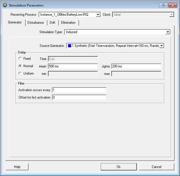
Figure 6.74: Induced Stimulation Scheme #
The following picture illustrates the two-step stimulus generation of an induced stimuli generator.
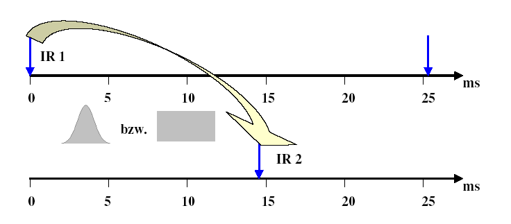
Figure 6.75: Induced Stimulation With Normal or Uniform Delay #
6.7.2.4.4 List Based #
The List Based stimulation generator allows adding stimulations as fixed points of time to a list of stimulations. As with the other stimulation types, a receiving target process has to be specified and optional disturbance and drift may be specified.
6.7.2.4.5 Induced List Based #
The Induced List Based stimulation generator is similar to the List Based stimulation generator. In the same way a list of discrete time points is managed at which the target is stimulated. Additionally a source generator has to be selected. Every the source generator stimulates its target, the list of time points is processed. If there are already stimulations from previous processings the new stimulations are added.
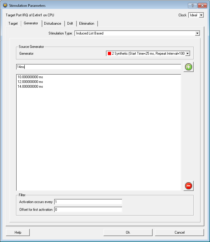
Figure 6.76: Induced List Based Generator #
An induced stimulation is specified as follows:
-
Select Induced List Based from the drop-down menu Stimulation Type.
-
From Source Generator select an already defined generator as the source of stimulation. Any other stimulation may be selected as source for induced list based stimulation.
-
Enter a Time value into the lineedit above the table and click (+) to add it.
-
Remove values from the list by selecting it and clicking on (-) to delete it.
-
Additionaly a period and an offset can be entered which are interpreted as a prescaler between the source generater and the induced list based generator.
As with the other stimulation types, a receiving target process has to be specified and optional disturbance and drift may be specified.
6.7.2.5 Stimulation Parameters - Disturbance #
Any stimulation generator may be subject to a random disturbance. Disturbances are parametrized with a probability of occurrence. The following image illustrates a stimulation disturbance:
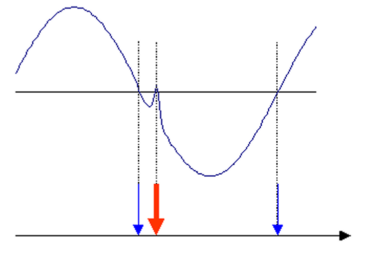
Figure 6.77: Example of Causal Stimulation Disturbance #
A stimulation disturbance is superimposed as follows:
Open the Stimulation Parameters dialog.
Select the Disturbance tab.
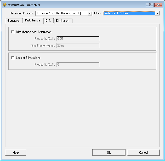
Figure 6.78: Disturbance Parameters Dialog #
Disturbance near Stimulation allows you to specify:
the Probability of disturbance occurrence and
a corresponding Time Frame.
Valid values for the probabilities are the range from 0 to 1.
Additionally with Loss of Stimulations you may specify
a Probability for the loss of a stimulus. Thus a probability of
1means "always lost" (disturbance never occurs) and0means "never lost"
6.7.2.6 Stimulation Parameters - Drift #
Stimulations may drift e.g. as result of deterioration or the impact of varying temperatures. You may also use drift to model a constant change rate of a stimulation (think of e.g. of a speed sensor of a vehicle in case of acceleration). To apply drift to a stimulation generator select the Drift tab of the Stimulation Parameter dialog.
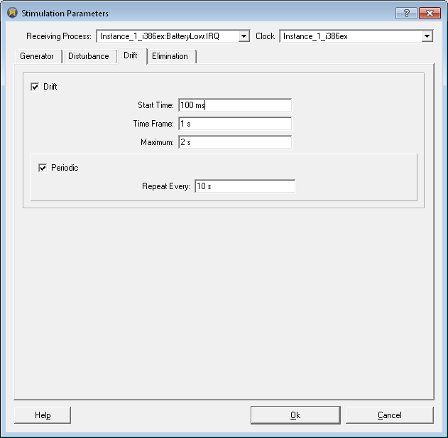
Figure 6.79: Drift Parameters Dialog #
The Drift tab allows you to specify
Start Time i. e. the time point when the drift starts,
the corresponding Time Frame (time period) of the drift. The drift will grow linearly as a function of time until the Maximum is reached and from there decreases linearly reaching zero at the given Time Frame
the Maximum value (reached at Time Frame / 2).
With Repeat Every an optional period may be specified to periodically repeat the drift characteristic.
The following picture exemplifies the effect of drift on the generator. Each time the drift value reaches the maximum value it is reset to grow linearly again from this point in time.
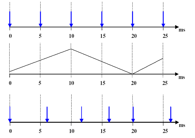
Figure 6.80: Drift of a Stimulation #
6.7.2.7 Limiting Stimulations with a Burst Filter #
A Burst Filter can be used to limit the number of stimulations a scenario can emit in a specified time period. It conforms to the AUTOSAR Burst Pattern.
6.7.2.7.1 Defining the Burst Filter #
Edit the scenario to which you want to apply a burst filter.
-
on
The Stimulation Parameter Dialog with the Burst Filter Settings opens.
Enter the values.
to close the dialog and to store the parameters.
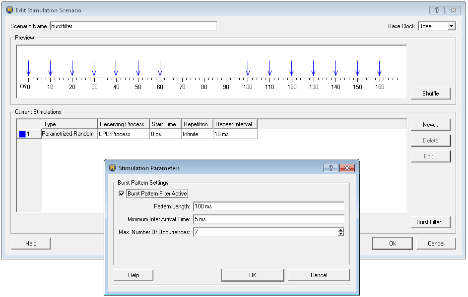
Figure 6.81: The Stimulation Parameters Dialog for a burst filter. #
6.7.2.7.2 Behavior the Burst Filter #
Figure 6.81, “The Stimulation Parameters Dialog for a burst filter.” shows an example of a burstfilter. The scenario itself is setup to emit a stimulation every 10ms. The burstfilter limits this to a maximum of 7 stimulations within 100ms. As a result the stimulations at 70ms, 80ms and 90ms are suppressed.
6.7.2.8 Stimulation Preview #
The result of your stimulation parametrization is displayed in the Edit Stimulation Scenario dialog. To get there open a project, select the module Stimulation and a scenario.
The Preview graph shows a random example instantiation of the scenario's stimulation generators as exemplified in the following image.
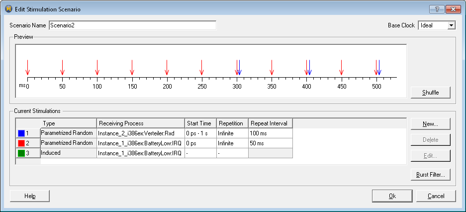
Figure 6.82: Scenario Preview #
The preview shows the stimuli as colored arrows on the time axis.
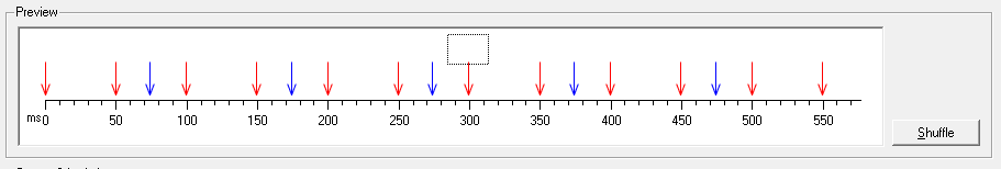
Figure 6.83: Stimuli Preview of a Scenario #
Each stimulus is shown in the color of its stimulation source. By ing an arrow the stimulus time (relative to simulation start) will be shown.
The button triggers the generation of stimuli for all defined stimuli sources. In case a generator has random parameters each application of will result in a different realization of the stimuli scenario.
6.7.3 Composite Scenario #
6.7.3.1 Defining a Composite Scenario #
6.7.3.1.1 Add a Composite Scenario #
In order to add a scenario, do the following:
Select the Module Stimulation
-
on
A new composite scenario is added to the model and the Composite Scenario Dialog opens.
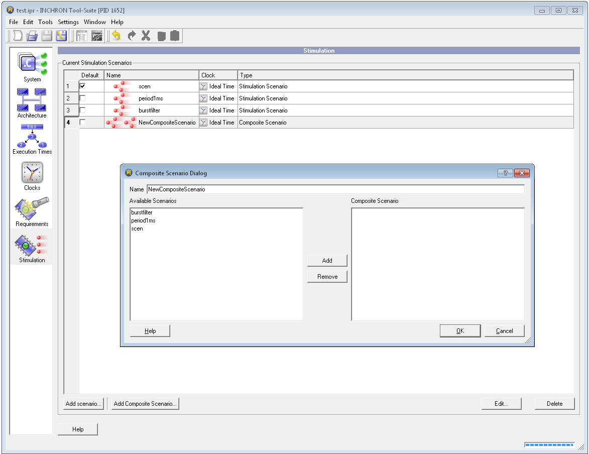
Figure 6.84: The Composite Scenario Dialog with a new composite scenario. #
Enter a name for the new composite scenario.
to confirm the changes.
6.7.3.1.2 Edit a Composite Scenario #
The scenarios in a Composite Scenario can be edited in the Composite Scenario Dialog.
Select the Composite Scenario you want to edit.
-
Either the scenario or on .
The Composite Scenario Dialog opens.
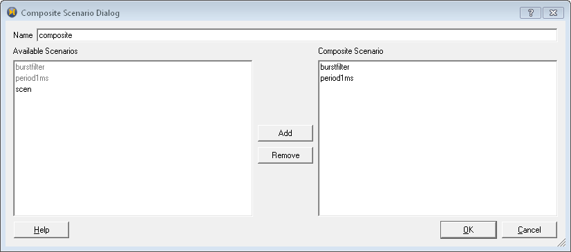
Figure 6.85: The Composite Scenario Dialog showing a composite scenario. #
-
Select an available scenario on the left side. to insert it into the Composite Scenario.
The contained scenarios are shown on the right side.
-
To remove a contained scenario on the right side, select it and .
The scenario is removed from the right side.
Press to confirm the changes.
6.7.3.2 Behavior of a Composite Scenario #
During simulation a Composite Scenario can be inserted into the simulated model like a normal scenario. The chosen start time is applied as start time to all contained scenarios.
All generators in a composite scenario are working independently of each other. Using the same target peripheral or process for different generators results in multiple activations and may lead to multi-activation errors depending on the properties of the activated process.
A composite scenario evaluates the contained scenarios independently from each other. If a scenario contains a burst filter (see Section 6.7.2.7, “Limiting Stimulations with a Burst Filter”) it is applied only to the stimulations of this scenario. Other scenarios may produce stimulations which violate the burst filter.
6.7.4 Import and Export of Scenarios #
A set of scenarios may be imported or exported.
Exported scenarios may be imported and applied to any project.
INCHRON scenario files have the file extension ISL (INCHRON Scenario List).
The scenario import from IPR file (INCHRON Project File) is also supported.
6.7.4.1 Scenario Import #
Importing a scenario is done with an import wizard which allows the selection of individual scenarios and assists you in targeting the stimuli generators to ports of the system model's peripherals.
Important:
In order to attach stimulation scenarios to peripheral ports or processes (or ISRs) during scenario import you may add the target peripherals and processes before starting the scenario import wizard.
In order to import a scenario, do the following:
Select → from the menu.
This will start the Import Scenario wizard.
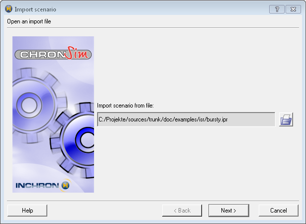
Figure 6.86: Initial Page of the Scenario Import Wizard #
Select the file to import the scenario from. You may import from INCHRON project files (
IPR), which already contain scenarios or from previously exported scenario files (ISL). Confirm your file selection with .The next page of the wizard shows a list of available scenarios.
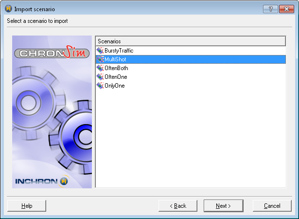
Figure 6.87: List of Importable Scenarios #
If the intended scenario is not listed in the selected file, you may return to the previous wizard page by clicking and select a different source file, or abort with .
Pick one or more scenarios from the list you may wish to import and continue with .
The next wizard page shows the mapping of the imported scenario's to your system's available processes and input ports. This allows a flexible adaption of the scenario to different CPU and peripheral targets.
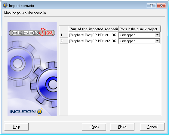
Figure 6.88: Mapping of Scenarios to Ports and Processes #
If your system's components exhibit the same target ports and processes contained in the imported scenario, the scenarios automatically be mapped to the respective targets.
Use the drop-down lists in the cells of the Ports in the current Project column to connect the ports of the scenario to the ports of your current project.
All ports must be mapped to your system's input ports.
If necessary, pick a different name for the scenario to be imported.
A scenario's name must be unique for a particular project. If a scenario with a given name already exists, you will get notified. In this case, simply pick a different name for the imported scenario and continue.
Click to start the scenario import.
The selected scenarios are now being imported and integrated into your current project according to your specifications. The wizard will now display its final page.
the wizard.
6.7.4.2 Scenario Export #
INCHRON Tool-Suite allows you to export a stimulation scenario to an INCHRON
Scenario List (ISL).
Scenario list files contain selected stimulation scenarios along with a short peripheral specification,
to allow for automatic remapping of ports on re-import.
That way you can use scenarios from one project for any other projects,
without disclosing details about your project’s processes, functions
and their mapping to resource and their execution times.
In order to export scenarios select
Select → .
The scenario export dialog appears, showing a list of exportable scenarios.
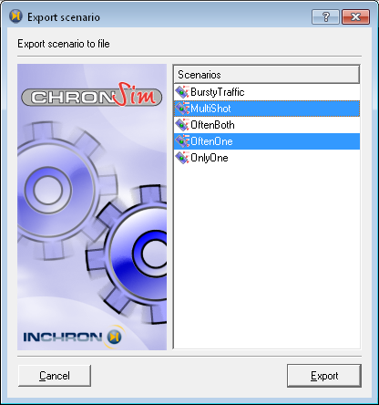
Figure 6.89: Scenario Export Dialog #
You may as well select one or more scenarios from the Module Stimulation in the project window. To do so, activate the context menu in the scenarios list by pressing the right mouse button and select Export Scenarios. Select one or more stimulation scenarios you wish to export from the list.
Confirm your selection with .
A dialog appears asking you for a file name for the exported scenario file.
Pick a file name and folder you wish to save the exported scenarios to. Finish the export of scenarios with , which will save the selected scenarios to the given file.
[1] See Reference Manual of Macros and Functions which is available via the Tool-Suite's help menu.
[2] See Reference Manual of Macros and Functions which is available via the Tool-Suite's help menu.
[3] In chronVIEW mode editing of requirements is only supported by invoking the model editor window like described in Section 3.2.5, “The Viewer Mode”. Event Timing Requirement.
[4] Specifying a requirement for a minimum execution time is possible by means of the more general Event Timing Requirement.
[5] in regular expression syntax "."
denotes any character, with modifier "*"
denoting any number of repetitions of "." (any character)
[6] Load requirements on LIN buses are not supported in Tool-Suite 2.6
7 Simulation #
This chapter will give you an introduction to the handling and user interaction of the Tool-Suite application when running a chronSIM simulation. For a better understanding, all explanations refer to one of the example simulation projects which are part of the Tool-Suite distribution. You can open an example project with →
This user manual can only provide an exemplary introduction on employing the chronSIM real-time simulator, hinting at how to use the simulator with its analysis tools for your special purposes.
For that reason an interpretation of or comment on the example simulation projects will not be given. This chapter will confine to the most relevant interaction steps of the INCHRON Tool-Suite concerning the following aspects:
The project description as a virtual hard- and software-model
Controlling the simulation
Visualization of simulation results
the verification of requirements
Loading and saving of simulation runs
Input scenarios for simulations
Exporting stimulation data
Report generation as interface to the documentation of the development process
7.1 The Simulation Concept #
During the simulation the chronSIM Real-Time Simulator window is visible. This window is used for controlling and analyzing simulation runs. The available simulation diagrams aim to present a thorough insight into different aspects of the dynamic behavior of a your simulation model. The user may select arbitrary time sections of the simulated system in each diagram for a closer inspection of the system's behavior.
The simulation itself is controlled by the user. Apart from starting, stopping, pausing and continuing the simulation, previously defined scenarios can be loaded and applied to the running simulation, acting as external stimulation.
A simulation run will allow you to analyze the system to give you a deeper insight into the following key questions concerning your system:
Is the system under examination properly specified?
Is the system generally able to meet the application's requirements?
Can tasks be optimized?
What timely behavior does the system have?
How does the system react to external stimulation?
The simulation aims to present a thorough insight inside the dynamic behavior of your target system. The simulation results offer a starting point and many hints to optimize the hard- and software of your target.
Many modifications on your system, like altering task priorities or a resource's scheduling strategy, can be edited via graphical dialogs without having to modify a single line of source code. For a modification to take effect in the simulation, the simulator must be restarted. Close the Real-Time Simulator window and click on the simulator icon in the project window toolbar in order to restart the simulation.
7.1.1 Toolbars #
The Tool-Suite application's provides convenient means for controlling the simulation via the toolbars of the chronSIM Real-Time Simulator window. The toolbars can be dragged away from the window docking position and dropped at arbitrary positions on your screen.
Toolbar Control
Simulation control operations: Run, Step, Break and Stop.
Toolbar Diagrams
View and hide the process state diagram, sequence diagram, event chain diagram, histograms, box plot diagrams, load diagram, stack diagram, and the function nesting diagram. Additionally the buttons to sync all diagrams and the live capture button are contained in this toolbar.
Toolbar Operation
Manipulation of the visual appearance, including zoom, height, granularity and smoothing of simulation diagrams.
Toolbar File
Loading and saving simulation results and editing of realtime requirements. Note: Additional functionality including several import and export options is available from the menu.
7.2 Running a Simulation #
A Simulation can be run in several modes.
The simulation runs continuously until it is stopped by hand or by a predefined event.
The simulation runs in step-mode which means it runs until the next simulation event occurs. The simulation stops immediately after each simulation event.
A simulation may be stopped, e.g. to perform a detailed analysis of task states, stack usages or communication relationships.
Analysis of a saved simulation result from a previous simulation run.
With the help of stimuli scenarios defined in module stimulation the effect of external signals may be studied.
With breakpoints (see Section 7.3, “Automatic Breakpoints”) the simulation may be stopped on events or on violation of functional or timing requirements
The functions of the menu allow you to trigger a single stimulus or to activate a complete stimuli scenario for a simulation run.
The Simulation Control window allows you to specify breakpoint conditions.
During simulation the current simulation time is shown and recorded. This is always simulated target time and has no relation to the host's time.
7.2.1 Starting a Simulation #
Load the example project
dect.iprfrom thedectsubdirectory.If the Tool-Suite is not yet running you may just double-click on the IPR file.
Otherwise If the simulator window is still open, you will get a warning message before the new project will be loaded.
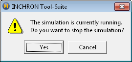
Figure 7.1: Warning in case of running simulation #
Confirm this message with or abort with .
If there are yet-unsaved modifications to your previous project, you will get another warning message to save your modifications to the project file.
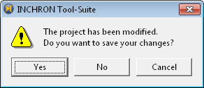
Figure 7.2: Warning in case of modified project #
Confirm this message with in order to leave the example project unchanged.
If necessary select the project
dect.ipr.Start the chronSIM simulation by clicking the corresponding
 icon from the toolbar.
The simulation executable will be generated. When finished the chronSIM Real-Time Simulator window will appear.
In order to watch simulation progress open one or more simulation diagrams.
You can start the simulation by clicking on
Run Simulation.
The status bar of the chronSIM Real-Time Simulator window displays the current simulated time on the target.
The simulation will run until reaching a breakpoint or being stopped manually.
Adjust the diagram axis scalings according to your requirements.
7.2.2 Step into Simulation #
Open a Diagram of your choice.
The respective diagram window appears.
Start the simulation by with
.The Simulation runs until either the next simulation event is encountered or a breakpoint is reached. The time indicator will show the elapsed target simulation time. .
At least one diagram window must be opened to see the simulation results.
Open additional diagrams at your choice.
Adjust the diagram views by scaling the time and result axes according to your requirements.
Another click onto will continue simulation until the next simulation event and so on.
7.2.3 Break into Simulation #
With
a running simulation will be stopped (paused).
The time indicator in the status bar will show the elapsed target simulation time.
In order to resume (starting from the current simulation time) use or .
The simulation time indicator will proceed from the already elapsed time.
7.2.4 Terminating a Simulation #
The  button terminates the simulation.
The simulation can be restarted from with or .
button terminates the simulation.
The simulation can be restarted from with or .
7.2.5 Simulation Events #
Events occurring during chronSIM simulation are recorded in the simulation trace file and shown in x/t diagrams. Simulation Events resemble a form of instrumentation which may be used to define automatic simulation breakpoints (see Section 7.3, “Automatic Breakpoints”). Simulation Events may be evaluated in timing requirements (see Section 6.6, “Module Requirements”) or histograms (see Section 7.7.11, “Histogram”) .
chronSIM differentiates between implicitly generated events and user defined (explicit) events. The following implicit events are provided by chronSIM:
entry and exit for functions,
start, end and fire for interrupt service routines (ISR),
activate and terminate for processes and OSEK tasks respectively
block, release and restart for processes and OSEK tasks: [7]
The block event occurs when a process enters the waiting state.
The release event occurs after a waiting process becomes ready.
The restart event occurs after formerly waiting process becomes running again.
Tip:
Time intervals between restart and block events are useful for measuring response times of extended tasks, and may be evaluated as Timing Requirement or as Histogram.
Explicit events are defined by instrumentation of the source code of the simulation model
using the EVENT() and EVENT1() macro.
For details refer to the application note Reference Manual of Macros and Functions
which is available via the Tool-Suite's help menu.
7.3 Automatic Breakpoints #
Using the → menu item you can raise and hide the Simulation Control window.
The Simulation Control window allows you to define conditions to automatically stop the simulation stop on certain system events. This includes violations of functional and real-time requirements as well as event and time based breakpoints.
Modifications in the Simulation Control window must be confirmed by clicking in order to take effect.
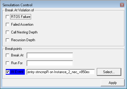
Figure 7.3: Simulation Control Window #
7.3.1 Breakpoint Criteria #
The following criteria are available for functional breakpoints:
stack overflow
limits on recursion and function nesting depth
RTOS violations, e.g. max. number of task activations (OSEK)
The stack size of each process is specified in the specification module.
If an option is deactivated (grayed out) in the Simulation Control window this indicates that the corresponding requirement is not specified and therefore not available as condition for a simulation breakpoint.
Additionally time or event based breakpoints may be set in order to make the simulation stop at
a specified absolute or relative simulation time
at entry or exit of a C function
on a specified interrupt
at the next occurrence of a user defined event specified in the C source code.
(see also Section 7.2.5, “Simulation Events”).
7.3.2 Time Based Breakpoints #
Defining a time based breakpoint requires specifying a time value and time unit. The Tool-Suite model editor accepts the following time units:
Table 7.1: chronSIM Time Units #
notation | unit |
|---|---|
s | seconds |
ms | milliseconds |
us | microseconds |
ns | nanoseconds |
ps | picoseconds |
T or C | clock cycles |
Check the box Run For.
In the input field enter a target simulation time of
200 ms.Confirm the new breakpoint with .
Start the simulation.
The simulation stops when the specified simulation time has elapsed.
The causing breakpoint condition is highlighted in blue in the Simulation Control window.
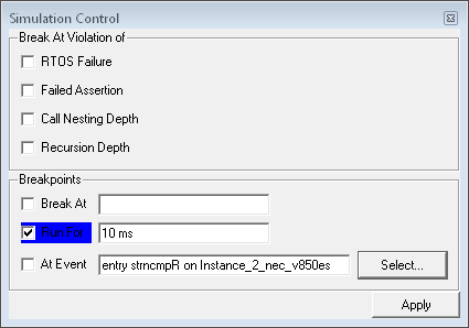
Figure 7.4: Simulation stopped by breakpoint #
Check Break At and enter
78 msinto the input field.Confirm with .
In this case you will get an error message, since the current simulation time is already past the value specified for Break at".
Correct the Break At value to
278 ms.Start the simulation.
The simulation stops automatically after reaching the given simulation time.
Experiment with arbitrary combinations of breakpoints. Restart the simulation after each modification.
7.3.3 Event Based Breakpoints #
With the At Event option it is also possible to automatically stop the simulation on a specified implicit or explicit (instrumented) simulation event. See Section 6.6.7.1, “Object Selection Dialog” for a description of the Object Selection dialog
7.3.4 Break at Requirement Violation #
In case Real-Time Requirements are defined for the project to be simulated,
it is possible to automatically stop the simulation on each violation
of certain types of requirements.
For demonstrating breakpoints on requirement violation the
dect_scenario,ipr example from the dect
subdirectory has to be used.
This project differs from the dect.ipr example project in
that limits are added on the stack usage, on function call nesting and recursion.
Load the
dect_scenario.iprexample projectWait until the chronSIM Real-Time Simulator and Simulation Control windows appear.
Select the Sequence diagram from the diagram menu.
The empty Sequence Diagram window opens.
If the Simulation Control window is not visible, you may use the → menu item to make the window visible.
Place the Simulation Control window outside of the chronSIM Real-Time Simulator window.
Start the simulation by with .
Without any breakpoint applied the simulation will run for
5 minutestarget time and beyond.Watch the evolution of the system in the sequence diagram.
Use the variable scales of the time and event axes to optimize the views.
Hide and re-enable the graphical elements of the sequence diagram.
Stop the simulation with when you feel confident with the view of your simulation.
Check all checkboxes listed under Break At Violation of
Confirm your modifications with
Start the simulation.
After some seconds of simulated target time the simulation stops due to violation of maximum call nesting depth.
The functional requirement that caused the break is highlighted in red in the Simulation Control window.
Experiment with arbitrary combinations of requirements. Restart the simulation after each modification.
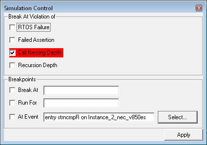
Figure 7.5: Simulation Stop Due to Requirement Violation #
7.4 Environment Variables #
Environment Variables are similar to the environment variables of a command line shell: They are stored outside of the simulated system, are available for every simulated process of the system, and are intended for passing values between the simulation control and the simulated system. They also share the same value semantics: they can be undefined (unset), defined but empty, or defined with a string value. Any of these manipulations may take place at any time during simulation.
Environment Variables can be used for the following features:
Usage and manipulation in the simulation model source code
Manipulation from the simulation control
Visualization in the simulator window
In case the value can be interpreted as an integer, the variable can be visualized using an analog meter meter (gauge) or a bar chart
7.4.1 Environment Variables in the Simulation Control #
Environment variables are controlled by the Environment Variables Window which is a modeless dialog from the Simulation Window. If it is not visible show it by selecting → . It can be hidden by the same menu item.
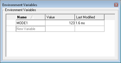
Figure 7.6: The Environment Variables Window #
To add a new environment variable click into the field containing New Variable and enter a name for your variable. Press enter to finish the entry. Now you have a new variable which is defined but empty. By continuing the simulation, the creation of the variable is applied to the simulated system and is available there.
Each environment variable is shown in a single line, containing its value (if set) and the timestamp of the last change. Variables which have been removed are shown in a strike-through font. Any changes which have been acknowledged by the simulated system will be shown with an animation. This allows the user to differentiate between recently created variables, changes of their values, and removals. After the animation of removals the corresponding line will disappear from the variable view, if the variable is not persistent.
Value changes for environment variables are simply entered in the column labeled Value and are acknowledged by pressing return. Changes take no effect until the simulation is continued, which allows to change more than one value at a time.
When moving the mouse pointer over an environment variable a
 symbol for a context menu appears
in the first column of the Environment Variable Window.
To remove an environment variable (to unset it) select
from this menu.
symbol for a context menu appears
in the first column of the Environment Variable Window.
To remove an environment variable (to unset it) select
from this menu.
Usually all environment variables are cleared at simulation start. If you want to set an environment variable to a specific value before the start of the simulation, you have either define it as a stimulation generator in the current stimulation scenario (see Section 6.7.2.2, “Stimulation Generators”) or mark it as persistent. To mark an environment variable as persistent, open its context menu and select . Persistent environment variables keep their last value over the restart of the simulation and are marked with a small icon.
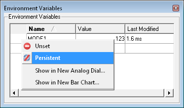
Figure 7.7: Persistent and non-persistent Environment Variables #
7.4.2 Environment Variables in the Simulated System #
The current status and value of an environment variable is accessible from the source code executed in the simulated processes. The programming interface offers these functions:
-
int isEnvironmentSet(const char* name);Returns 1 if the environment variable with the name name is set.
int getEnvironmentInt(const char* name, int* value);Returns 1 if the environment variable name is set and can be converted to an integer value. In case of success the integer value is stored in the variable value.
void setEnvironmentInt(const char* name, int newValue);Sets the environment variable name to the string representation of the integer value newValue.
int getEnvironmentString(const char* name, char* value, unsigned int maxLen);Returns 1 if the environment variable name is set. The first maxLen-1 characters are stored at value and terminated by a zero. In case of an environment variable which is set but has no value a single zero is stored in value.
void setEnvironmentString(const char* name, const char* newValue);Sets the environment variable name to the string value newValue. The string must be zero-terminated. A value of zero for newValue means to unset the environment variable. A zero-length string (newValue pointing to a single zero) means that the environment variable is set but has no value.
The value of environment variables can be used to control the behavior of the simulated system, for example execution times can be scaled by a value given from the outside. It can also control mode dependent behavior as well as giving set values for processes replacing environmental behavior.
7.4.3 Visualization of Environment Variables #
If an environment variable takes integer values, its current value can be visualized with two views: an analog meter (gauge) or a Bar Chart. Multiple environment variables can be combined in a single diagram.
To show an environment variable in a diagram open the its context menu and select or .
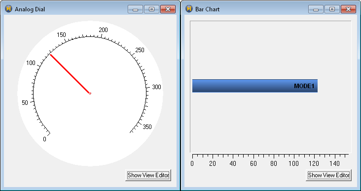
Figure 7.8: Persistent and non-persistent Environment Variables #
7.5 Stimulation #
In simulation mode there are two ways for stimulation:
manual single stimulation
stimulation using scenarios
Continuous stimulation by stimuli scenarios may be arbitrarily mixed with manual single stimuli at any time during simulation.
7.5.1 Manual Stimulation #
By applying a single stimulus you may either
trigger an interrupt or
send a signal to the input of a peripheral component at a specified point in time.
Activate a single stimulus as follows:
Procedure 7.1: Configuring Manual Diagram Scale Range #
Start a project in simulation mode
From the menu choose →
The dialog Specify a Single Stimulus pops up
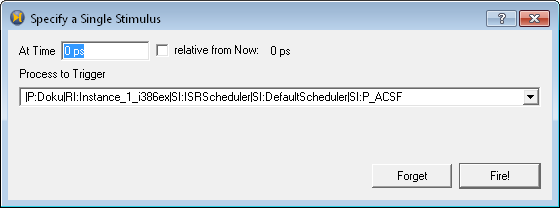
Figure 7.9: Single stimulation Settings #
Specify the point in time At Time of the stimulus.
Choose the target (IRQ or peripheral component) with Process to Trigger
Optionally with Relative from Now you may mark the point in time as relative to current simulation time.
Activate your setting with Fire! or cancel with Forget.
7.5.2 Applying a Stimulation Scenario #
Load the
dect_scenario.iprexample project from thedectsubdirectoryStart simulation mode
Open the scenario dialog with → → .
The Insert Stimulation Scenario into Simulation dialog opens.
If a scenario is already activated you have to remove it with → → .
Now select a predefined scenario from the e.g. Scenario1
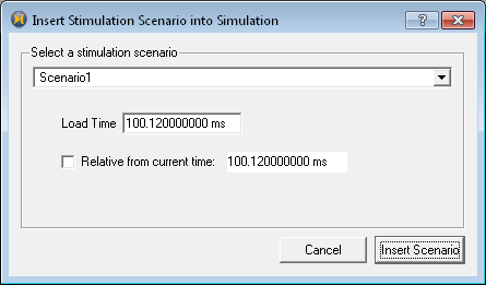
Figure 7.10: Loading a Scenario #
With Load Time specify the time on which the stimuli of the scenario should start.
Alternatively you may specify a time relative to the current simulation time by checking Relative from current time
Confirm your settings with or choose .
The status bar of the chronSIM Real-Time Simulator window will show the Name of the activated scenario.
7.6 Real-Time Requirements #
Section 6.6, “Module Requirements” describes, how application specific real-time requirements are defined for a system model. In simulation mode the Requirement-Editor is shown as a separate window, allowing editing of requirements and their properties at any time.
The requirement view in simulation mode shows the current evaluation counts and resulting evaluation status of all requirements. After simulation start the requirement window will be continuously updated. Beside evaluation count each requirement visualizes its resulting evaluation verdict with a green, yellow or red icon.
Tip:
The simulation time range considered for requirement evaluation may be limited with the global time range filter
Via the Enabled and Show columns of the requirements window the evaluation and the visibility of their evaluations in diagrams respectively may be controlled for individiual requirements and requirement groups.
Note:
After editing a requirement it will be automatically re-evaluated. An incomplete state of requirement evaluations is indicated by temporarily showing a requirement's evaluations counts in grey color.
With → the contents of the requirements editor window may be exported as image.
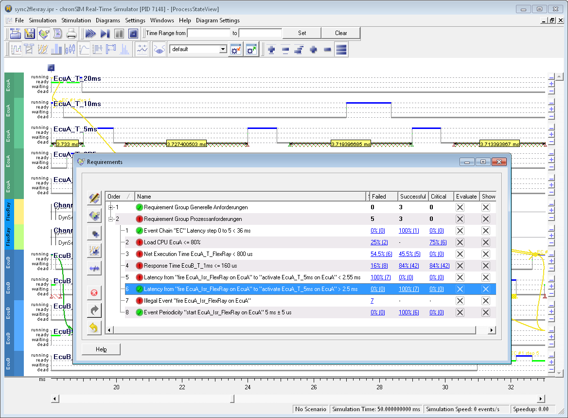
Figure 7.11: Overview Requirement Evaluation #
Load the example project sync2flexray.ipr
and run the simulation for 50ms.
Open the requirement editor with
→
or use the respective toolbar icon.
The project's requirements are structured in two main requirement groups, as shown in the Requirements window. For each requirement the columns Failed, Critical and Successful show the corresponding evaluation counts. A colored icon in the Name column gives a quick indication of a requirements resulting evaluation state (verdict):
In case of no evaluations a gray icon is shown.
In case of failed evaluations a red icon is shown.
In case of no failed but critical evaluations a yellow icon is shown.
In case of only successful evaluations green icon a shown.
For requirement groups these columns comprise the results of the contained requirements as follows:
A red icon (failed) is shown if at least one of the group's requirements is failed.
Column Failed shows the number of failed child requirements
Accordingly column Successful and Critical show the number of child requirements which which evaluate as Successful or Critical.
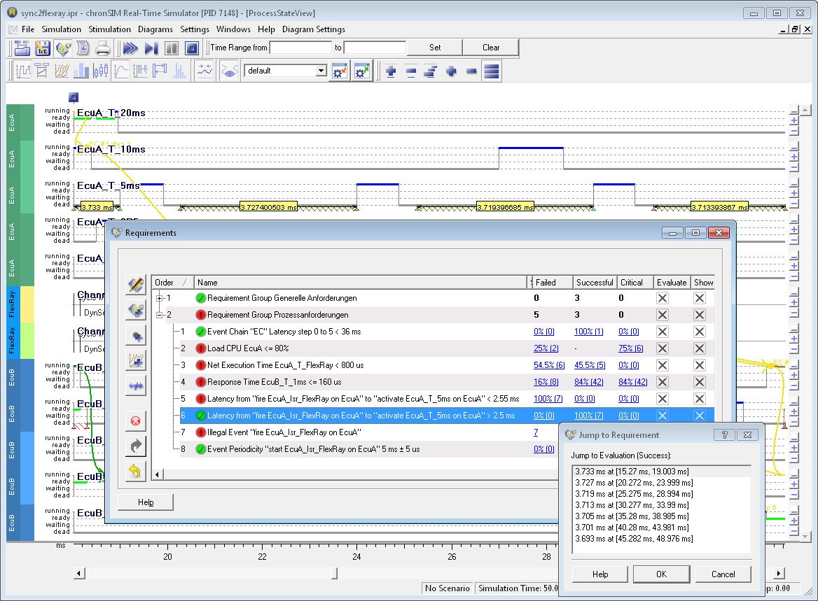
Figure 7.12: List of Requirement Evaluations #
A list of all evaluations of a requirement is shown by a verdict count in one of the evaluation columns Failed Critical of Successful. The Jump to Requirement window lists the time intervals of the events evaluated by the requirement.
Jump to Requirement Evaluation#
By an entry in the list of time intervals the time axis of open x/t diagrams will be scrolled to this interval. Figure 7.13, “Jump to Requirement” shows the evaluation of a Response Time requirements in the process state diagram.
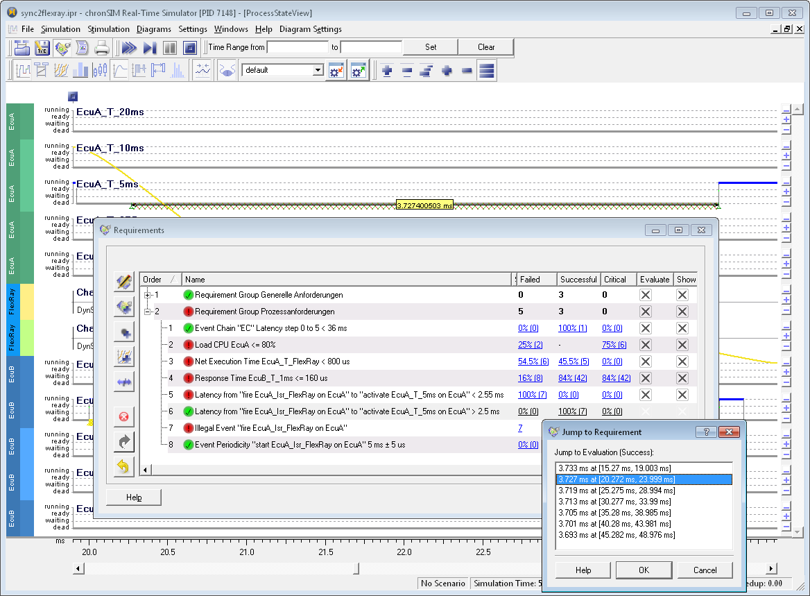
Figure 7.13: Jump to Requirement #
7.6.1 Statistics on Timing Requirement Evaluations #
In contrast to functional requirements the evaluation of timing requirements is always based on a time measurement. Using histograms it is possible to analyze the time distribution for evaluations of a timing requirement.
The requirement reporting functionality of the Tool-Suite will also include histograms of timing requirement evaluations and statistical information (min., max., average value).
7.6.2 Export and Update of Requirements to DOORS #
After simulation or validation the state of the requirement evaluation can be exported to a DOORS database. See Section 11.2.4, “Export and Update of Requirements to DOORS” on how to perform the necessary steps.
7.7 Visualization #
- 7.7.1 Time Range Filter
- 7.7.2 View Profiles
- 7.7.3 Statistics View
- 7.7.4 Diagram Types
- 7.7.5 x/t Diagrams
- 7.7.6 Diagram Usage
- 7.7.7 State Diagram
- 7.7.8 Gantt Diagram
- 7.7.9 Sequence Diagram
- 7.7.10 Event Chain Diagram
- 7.7.11 Histogram
- 7.7.12 Box Plot Diagram
- 7.7.13 Load Diagram
- 7.7.14 Stack Diagram
- 7.7.15 Event Diagrams
- 7.7.16 Nesting Diagram
- 7.7.17 Console View
INCHRON Tool-Suite provides different types of diagrams for the visualization of the dynamic system behavior, e.g. for viewing process states or resource loads over time, histograms, a box plot of process response times and a statistics view.
All diagram windows can be viewed from the Real-Time Simulator window, which becomes available when starting a simulation or loading a previously saved simulation trace file.
You may switch between defined sets of view windows, by defining View Profiles, as described in the following section
Additional diagram functionality for printing or exporting data can be accessed via the menu bar or the context menu.
7.7.1 Time Range Filter #
Several aspects of visualizing and evaluation of simulation data may be restricted to a globally set time range. The Time Range Filter may be configured with the following steps:
Click the corresponding toggle button in the simulator window's toolbar.
This will invoke a time range input dialog. Leaving the first time input field empty will be interpreted as a start of the time range and
0ms. Leaving the second time input field empty will be interpreted as current end of simulation.The global time range filter may be disabled by clicking the corresponding icon in the simulator window's toolbar.
For re-enabling click the icon again and just press enter to confirm the current time range setting.
The filter will affect the evaluation time range of histograms, requirements, the statistics view and reporting.
7.7.2 View Profiles #
The Simulator Window allows to define any currently shown set of open views as a view profile.
You can define multiple named view profiles and conveniently switch between them.
Defined View Profiles are persistently stored
any time you write your project to the IPR project file.
7.7.2.1 Switching View Profiles #
The view profile selection drop-down list in the diagram toolbar shows the name of the current view profile and allows for conveniently switching between defined view profiles. This requires the definition of at least two profiles, as described in the next section.
Important:
Selection a different view profile will discard any unsaved changes of the currently active view profile and will switch to the last stored state of the selected view profile.
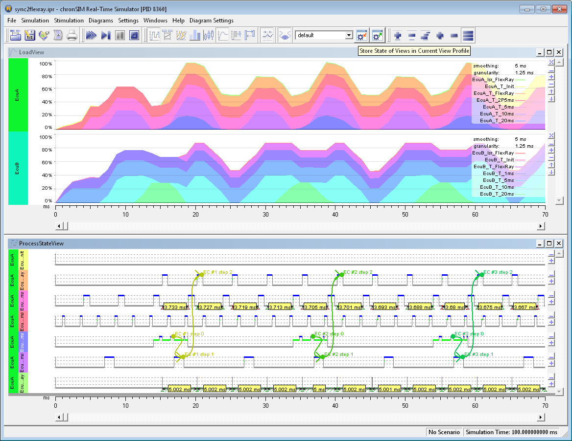
Figure 7.14: View Profile Controls #
7.7.2.2 Storing and Restoring a View Profile #
Initially a simulation project has an empty default profile. Every view profile maintains a last stored state, which you can act on with the toolbuttons to the right of the view profiles drop-down list in the simulator window toolbar:
-
In order to store the current state of views to the currently active view profile, use the
 Store State of View Profile toolbar button.
 -
In order to restore (apply) the last stored state of the currently active view profile, use the
 Restore State of Views toolbar button.
Important:
Storing a view profile is persistent between invocations of the Tool-Suite simulation mode. However to make stored view profiles persistent between invocations of the Tool-Suite application, you have to save your INCHRON project to an IPR file (in the Tool-Suite application main window).
7.7.2.3 Defining and Managing View Profiles #
The special Edit View Profiles... entry of the view profile drop-down list will invoke the View Profile Dialog for managing defined view profiles. The View Profile Dialog allows the creation of a new profile and renaming and deletion of existing view profiles. Adding a new view profile will clone the state of the currently active view profile.
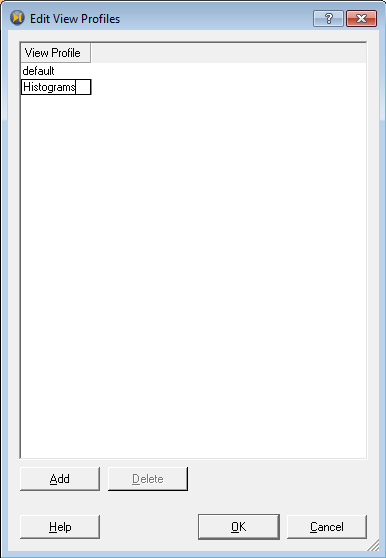
Figure 7.15: View Profile Dialog #
In order to define an additional view profile with two histograms as shown below, follow these steps:
Open the simulation window with the example project
sync2flexray.ipr.Close any diagram windows.
Run the simulation.
Add two histograms as described in Section 7.7.11, “Histogram” and place the histograms side by side.
Select Edit View Profiles... from the View Profiles drop-down list, which will invoke the Edit View Profiles Dialog.
Select Add and enter the name Histograms for the new listbox item.
After pressing OK the name of the active profile appears as Histograms as shown below.
You may now switch back to the default profile by selecting its name from the view profiles drop-down list.
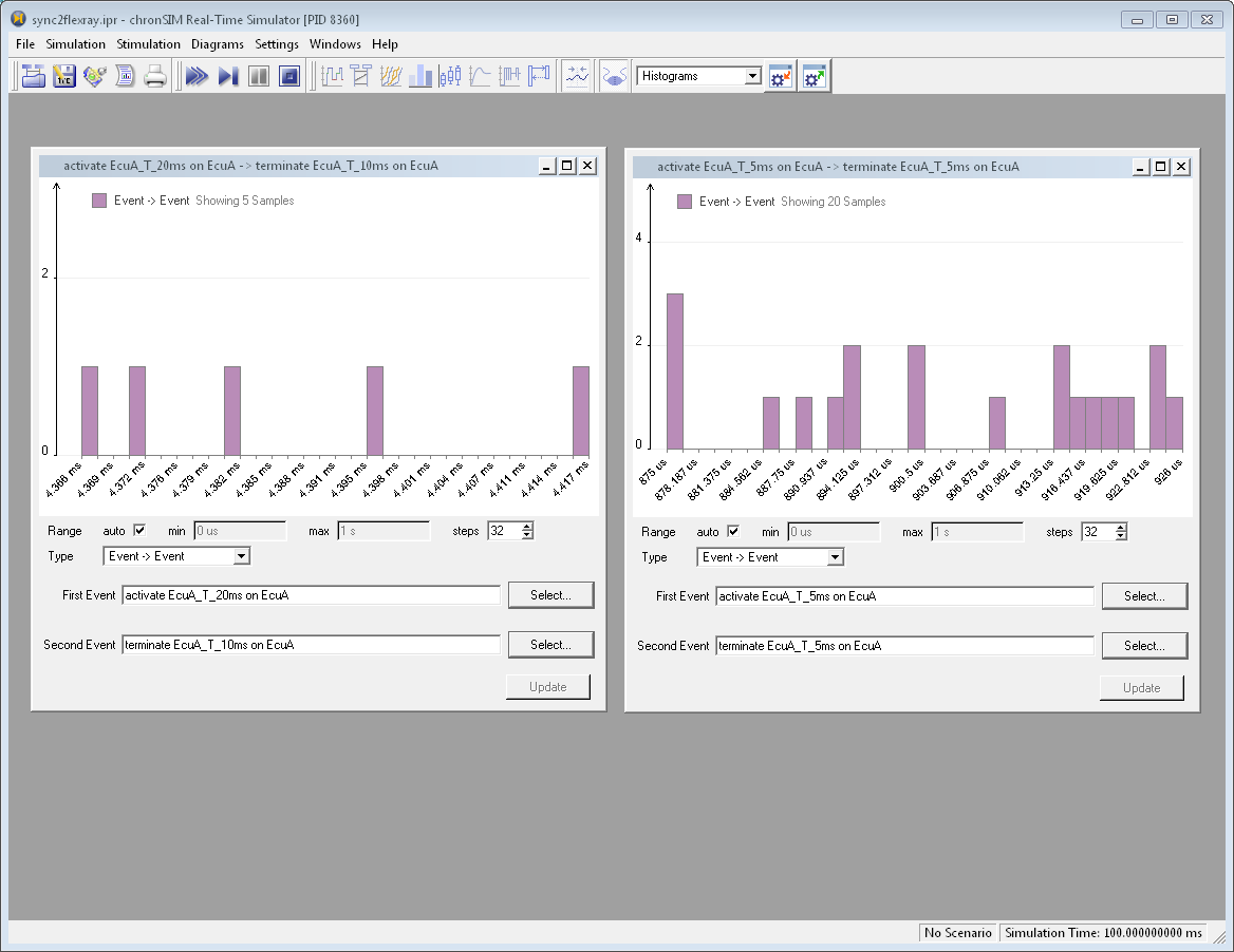
Figure 7.16: View Profile with two Histograms #
7.7.2.4 View Profiles and chronVIEW #
When working with saved simulation trace files
(ISF) or imported traces within
chronVIEW the same view profiles features as within chronSIM are
available. However when opening such a trace the state of the view
profiles represent the state of the view profiles in the project at the
time the trace was created. Additionally changes to view profiles can
not be stored in the trace.
Important:
Working with existing simulation trace files in chronVIEW
will leave the trace file (and its view profiles) unmodified.
Modified view profiles may be applied though by storing into a separate
IVP file.
To save changed view profiles you must use
→ . This stores the current state of the
view profiles in a separate file named as the trace with the file
extension IVP.
When opening a simulation trace, a file with the same name and the
file extension IVP in the same directory is searched.
If it exists contained view profiles are automatically imported.
Existing view profiles from the simulation trace (ISF) are overridden
by view profiles with the same name from the IVP file.
Copying view profiles between trace files is possible by simply copying and renaming IVP
files.
View profiles of an existing INCHRON project file (IPR)
may also be used for this purpose by copying and changing its file extension to IVP.
7.7.3 Statistics View #
The Statistics View shows on the fly statistics of process execution times, CPU and bus resource loads and rates of IPC operations (e.g. mutexes and semaphores).
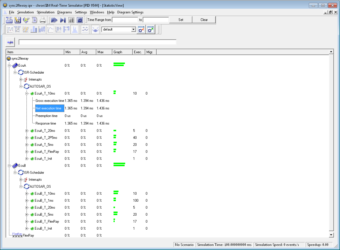
Figure 7.17: Statistics View #
Tip:
In case a global time range filter is active, the Statistics View will switch to show statistics over the whole global time range (instead of short time statistics), after the simulation time reaches the upper limit of the global time range filter.
7.7.4 Diagram Types #
All diagram windows can be displayed simultaneously. A Diagram window may be opened by using the tool buttons of the diagram toolbar or by using the menu. A diagram window usually comprises a set of diagrams of the selected diagram type for each process of the project (excluding idle tasks).
A diagram window may be closed with Ctrl–F4 (or Ctrl–W) or minimized. The arrangement and visibility of individiual diagrams may be manipulated by either mouse operations or more conveniently with the Diagram Order dialog.
The menu provides control of diagram visualization options which are dependent on the diagram type currently activated.
-
This diagram visualizes the timed sequence of
each tasks operating system states running, ready, waiting or dead and
messages of CAN and FlexRay communication buses
-
Sequence Diagram or communication activities.
This diagram shows communication activity between tasks as well as between tasks and ISRs.
-
This diagram shows graphs of Event Chain instances.
-
Shows the statistical distribution of the time interval of two events. Unlike other diagram types multiple histogram windows may be open at the same time.
-
Shows a box plot of process (and ISR) response times
-
Utilization of a microprocessor or bus resource.
-
This diagram shows rate, value and counter diagrams of system events (like EVENT1() macros), see Section 7.7.15, “Event Diagrams”.
-
This diagram shows the nesting depth of functions of a process.


7.7.4.1 Diagram Functions #
Functions for diagram handling are available in the menu and the diagrams context menus. The functions are diagram type specific.
The following functions are available:
Jump
Scroll time axis to
a given time,
to start of a requirement evaluation, or
to start of a CAN bus message (state diagrams only).
Print...
Print single or multiple diagrams of a diagram view
Export as SVG...
export as vector graphic (not histograms)
Export as CSV...
Export of diagram graph values comma separated values (x/t diagrams only but not the Load Diagram).
Move
Change diagram order in a diagram view (x/t diagrams only).
Close
Hide diagrams of a diagram view (x/t diagrams only).
7.7.4.2 Diagram Selection and Order #
Another way to arrange diagram order or select diagrams to be shown or hidden of any x/t diagram window is by using the Diagram Order dialog via → . The Change Visibility and Order dialog shows all available diagrams in two lists, with currently hidden diagrams shown to the left and currently visible diagrams to the right.
Usually items are presented hierarchically, with process items shown as children of their CPU resource.
For more flexibility on diagram order the hierarchical presentation of the list of visibile diagrams may be disabled using the Group by Resources checkbox.
In case of many diagrams the lists may be filtered by entering a search string in the Filter edit field.
Tip:
Double clicks on list items is sufficient for moving them between the dialog's lists:
Double clicking a process item will toggle visibility for the corrresponding process.
Double clicking a CPU item will toggle the visibility of all its processes at once.
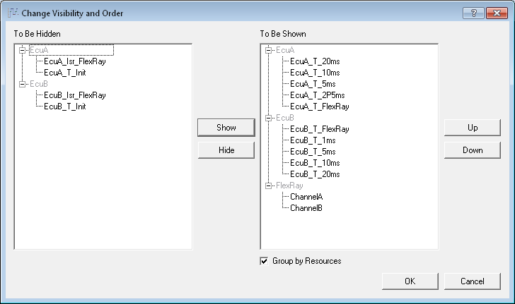
Figure 7.18: Diagram Order Dialog #
7.7.4.3 Printing and Exporting Diagrams #
Using the print or export functionality of diagrams from the file or context menu invokes the export options dialog. This dialog provides export options as shown in the image below.
Checking the Export Diagram Header option will add a descriptive header to the exported data containing meta data concerning the simulation project.
The buttons below the Time Range label may be used to define the time range of the diagrams to be exported.
For x/t diagrams the Diagram Selection allows you to specify whether one single diagram, all visible diagrams within the visible window or all diagrams should be exported.
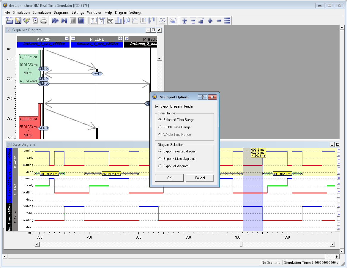
Figure 7.19: Options for Diagram Export #
Actual rendering of font sizes in exported SVG files depends on your viewer's settings. Using e.g. Mozilla Firefox-3, these settings can be altered via the → → → menu.
7.7.5 x/t Diagrams #
All diagrams except histogram, box plot and sequence diagram are x/t ("variable x over time") diagrams, i. e.
they show the graph of a simulation variable x over time t.
All x/t diagrams have a common base functionality described in this section.
7.7.5.1 Global Time Axis #
For each type of x/t Diagram the diagram view window shows multiple diagrams (e.g. for multiple processes) with a common time axis.
Changing the time scale affects each of the diagrams.
In order to rescale the particular diagram view
Then rescale the time axis by clicking on
 or
or  or button
in the Simulation window
toolbar until the desired scale of the diagram time axis is reached.
or button
in the Simulation window
toolbar until the desired scale of the diagram time axis is reached.
7.7.5.2 Continuous Update #
During simulation all x/t diagrams are usually continuously
updated to show the current end of simulation („Live Capture“).
In order to disable this feature the
 Live Capture toggle button.
7.7.5.3 Close Diagram #
Single diagrams of a diagram view may be closed with x
7.7.5.4 Move Up/Down #
Diagrams may be moved vertically in the Diagram view by either
drag-and-drop or with the
 arrow buttons on the right of each diagram.
7.7.5.5 Rescale y-Axis #
The height of each diagram may be enlarged or reduced individually
using the
 (plus/minus) buttons on the right of each diagram.
This will adjust the diagram's height.
(plus/minus) buttons on the right of each diagram.
This will adjust the diagram's height.
With the
Automatic Diagram Height button of the toolbar
the height of each diagram will be automatically adjusted
to fit all diagrams of the diagram window.
Note:
The Automatic Diagram Height feature is disabled whenever you manuall change the height of any diagram (or all at once with the Increase Diagram Height tool button).
7.7.5.6 Specify y-Axis Range #
Certain diagrams, i.e. the Load Diagram and the Event Diagrams support the manual setting of the y-axis range limits. The corresponding option is available from the context menu of the diagram's y-axis (see e.g. Procedure 7.2, “Adding Different Types of Event Diagrams” on how to add an Event Diagram):
Right click the diagram's y-axis to open the context menu.
From the context menu select
Result:The Configure Scale dialog opens.
Uncheck Auto range.
Adjust the Minimum value and Maximum value as required.
Confirm with .
Result:The diagram adjusts its scale range according to the specified limits as in the example below.
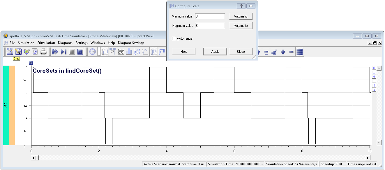
Figure 7.20: Manual y-Axis Range in Event Diagram #
7.7.5.7 Zoom - Region of Interest #
The time scaling of all x/t diagrams may be changed by using the mouse wheel in conjunction with the Ctrl key.
In some cases you may wish to examine a specific region of interest (ROI) of your simulation more closely, Such a region may be zoomed by marking the time range with the mouse:
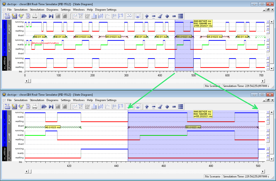
Figure 7.21: Zoom - Region of Interest #
If the simulation is running disable
Live CapturePress and hold the left mouse button and select a time region using the mouse
The ROI will be highlighted with light blue color.
Release the mouse button and click with the right mouse button inside the ROI.
The diagram context menu will be shown
Click the menu item.
The ROI is scaled to fit the whole diagram view width.
In case the you want to adjust the ROI anywhere outside the highlighted region in order
The highlighting gets discarded
You may now start over.
7.7.5.8 Reference Cursors #
A possibilty to measure distances is already shown in the section called “Zoom - Region of Interest”: On the top of the region the borders and the distance are shown. A better way to measure one or more distances is using the reference cursors.
Conceptually the reference cursors use a master cursor and one or more slave cursors. The time position of the master cursor is shown as an absolute value, while the time position of a slave cursors is shown relative to the master's time position, including a small arrow to indicate the relative position of the master.
A cursor can be added as follows:
-
Click on the reservoir on the top-left corner of a x/t diagram view and drag it to the right.
-
Drop it where the first measurement point is intended. This creates a new cursors which will automatically be the master cursor if it is the first cursor.
-
Repeat this for as many slave cursors as needed.
-
Adjust a cursor by dragging it to the left or right. When a cursor is dragged within a specific diagram, the cursor will snap on the next event in this diagram. When it is dragged in the area where the timestamps are shown, it will snap on the next event in any diagram.
Note: Timestamps of a slave cursor will not be shown if the distance to the neighbours is to small for the text. Zoom-in to see the values.
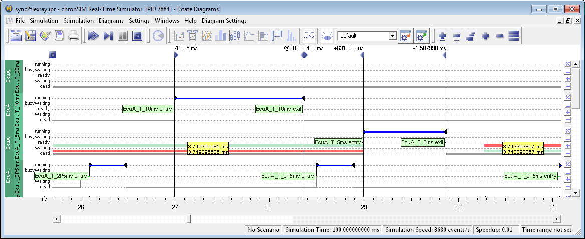
Figure 7.22: Reference Cursors #
7.7.6 Diagram Usage #
After this brief introduction to the basic features of the Tool-Suite's simulation visualizations you will now be introduced to each x/t diagram type's specific properties. To follow the instructions, you need to load and compile a simulation model in order to enter simulation mode:
Start the INCHRON Tool-Suite
Once the application has started load the example project
dect.iprThe project is being loaded.
Start the simulation mode by clicking the the
toolbar button.The chronSIM Real-Time Simulator window appears, accompanied by the Simulation Control window.
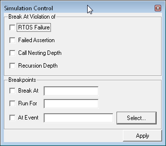
Figure 7.23: chronSIM Real-Time Simulator and Simulation Control Windows #
Now start the simulation by on the
toolbar button.
Since no diagram has been opened yet the only indication of the simulator being running is the simulation time indicator in the status bar.
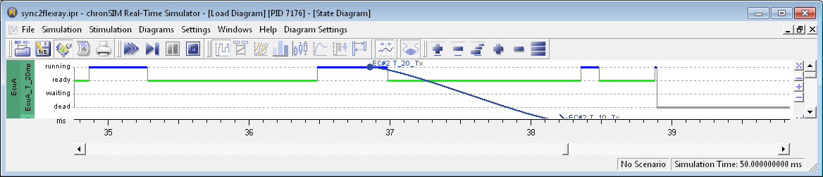
Figure 7.24: Status-Bar of Real-Time Simulator Window #
7.7.7 State Diagram #
the sequence of changes of operating system states for each task and
packets of communication buses.
7.7.7.1 Visualization of Task States #
All processes (with exception of idle tasks) and ISRs of a CPU resource are displayed as diagram in a shared window.
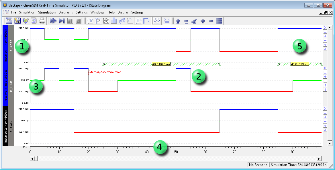
Figure 7.25: State Diagram of Example dect.ipr #
The numbered items in the picture above denote the following:
Task identifier
Operating system states of the task: running, ready, waiting or dead
Current state of the process
Simulation time axis
-
Evaluation of a real-time requirement. .
Note:
If case of tight vertical space for diagrams (e.g. in case of showing an unfiltered view of many processes), the presentation of individual state diagrams is automatically switched to the more terse gantt perspective.
7.7.7.2 Visualization of Bus Packets #
Communication packets between microprocessors are also shown in the State Diagram. For each channel of a FlexRay bus, for CAN or LIN bus, and for each link between an ethernet controller and an ethernet switch a separate line is drawn.
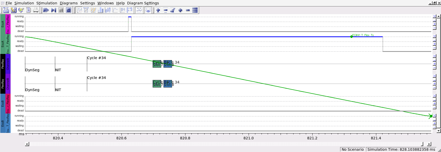
Figure 7.26: State Diagram showing packets on a FlexRay bus. #
The packets are always colored in the color of the origin, even when forwarded through an ethernet switch. Packets originating from the Restbus module are painted gray by default unless you activate → .
Depending on the type of communication bus extra information is shown like the arbitration phase of CAN packets, or the different phases of a FlexRay cycle (from an individual point of view from each controller.
7.7.7.3 Visualization of Event Chains #
If your project has Event Chains (which are visualized in the Event Chain diagram), these are also shown in the process state view as a graphical overlay as in the State Diagram). Event Chain steps are shown as bullets in the diagram of the originating process or bus.
In order to focus on specific chains of interest or even chain instances, it is possible to selectively filter Event Chains or Event Chain instances to be shown in the state diagram window via the Event Chain Visibility dialog. Invoke the Event Chain Visibility dialog with → .
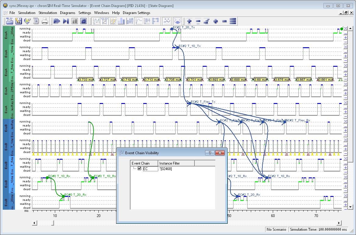
Figure 7.27: Event Chain Visibility Dialog #
The Event Chain Visibility dialog lists the project's event chains, which can be enabled or disabled globally with a checkbox. Alternatively, for event chains marked as shown you have fine-grained control over which chain instances to be shown be entering a regular expression in the Instance Filter column.
The image below shows the filtering of chain instances with even index by using the expression .*[02468].
[8].
You may use the expression 3|7|11 for showing only chain instances 3, 7 and 11.
The expression .*[05]00 will show only every 500th chain instance.
7.7.7.4 Visualization of Errors #
If your simulated system causes an error, each occurrence is indicated in the state diagram. E.g. if the simulated system accesses an illegal memory area, this will be flagged with a Memory Access Violation as shown in the next figure. For fixing such errors see the Edit Memory Dialog in Section 6.2.6.2.3, “Tab Memory Regions”).
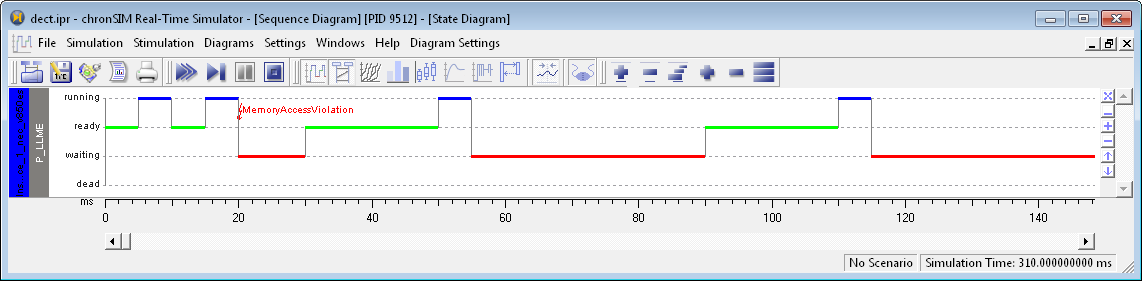
Figure 7.28: State Diagram with Memory Access Violation #
Other errors which are shown this way are an exceeded multi activation limit of an OSEK Task or lost interrupts, which are not handled by the processor.
7.7.8 Gantt Diagram #
The gantt perspective is an alternative view of the state diagram,
which focuses on visualization of process execution times,
bus message transmission times and activation dependencies.
If the Tool-Suite gantt chart license option is selected
you can switch the state diagram
to the gantt perspective with
→ .
The following two images show the original process state diagram
of the doc/examples/ethernet/taskmodel.ipr example project
and the the same view after switching to the gantt perspective.
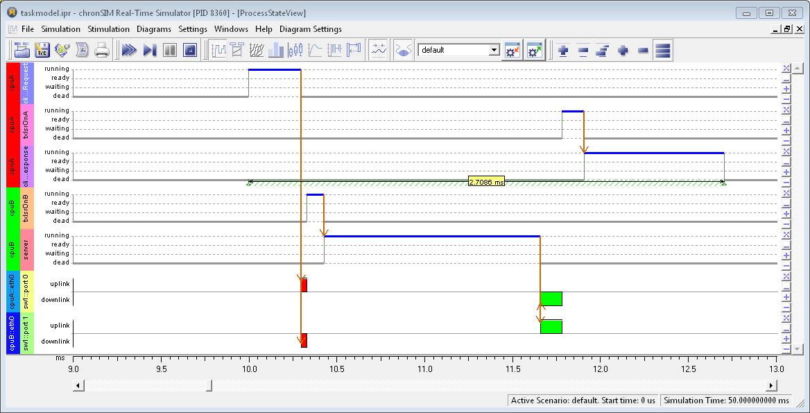
Figure 7.29: State Diagram of Example ethernet/taskmodel.ipr #
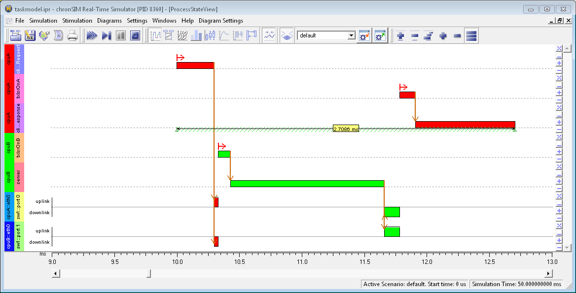
Figure 7.30: Gantt Diagram of Example ethernet/taskmodel.ipr #
Process states can be read from the Gantt chart as follows
A running process is shown as a bar in the color of the CPU resource,
a process in state waiting is shown as a pale colored bar and
a process in state ready is shown as a white colored bar.
Process activation dependencies are shown with red arrows between process bars. In the same way, processes modeled in a task model as triggering bus messages or vice versa are shown as arrows between processes and bus messages.
Displaying of labels of process activation and termination timestamps. This can be selectivel activated for individual processes with → as shown in Figure 7.31, “Show Process Details Dialog” and Figure 7.32, “Gantt Diagram with Process Details”.
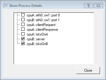
Figure 7.31: Show Process Details Dialog #
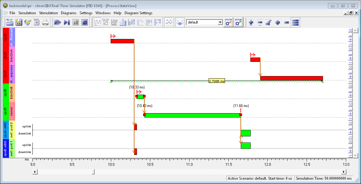
Figure 7.32: Gantt Diagram with Process Details #
7.7.8.1 Collating Processes #
An additional feature of the gantt chart view not available in the standard state diagram is the collation of processes into a single bar. This allows for showing either aggregated execution times of all a CPU's processes or for showing aggregated execution times of custom groups of arbitrary processes from one CPU:
All processes on a CPU resource may be collated with → .
Groups of processses from one CPU may be collated with from the process diagram context menu.
7.7.9 Sequence Diagram #
The sequence diagram visualizes the communication between tasks and ISRs (interrupt service routines). The diagram shows each task instance on its own instance axis. The busy times of a task or an ISR are displayed as bold lines on the vertical task instance axis. If your project has Event Chains (which are visualized in the Event Chain diagram), these are also shown in the process state view as a graphical overlay as in the State Diagram). Event Chain steps are shown as bullets in the diagram of the originating process or bus.
Open the sequence diagram by clicking on the
icon in the tool bar.
A window appears which displays the current simulation run.
Pause your simulation after about
250 ms.Adjust your diagram's settings so that your view of the diagram looks similar to the following image:
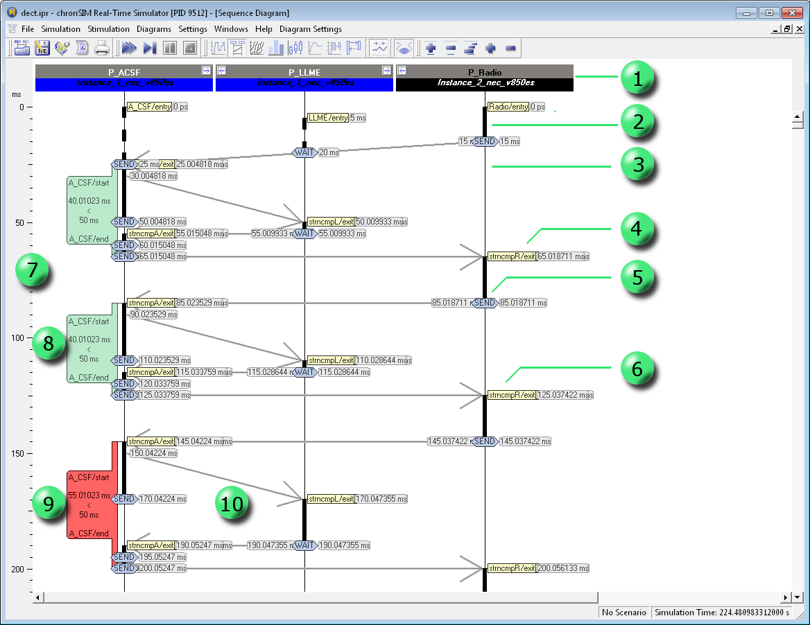
Figure 7.33: Sequence Diagram of Example
dect.ipr#
The items in the picture above have the following meanings:
Heading with Task and CPU resource identifier as specified in Module System. In this example task P_Radio on CPU Instance_2_i368ex
Bold line: indicates the task is being executed.
Thin line: The life axis ("lane") of a process.
An Event of a Task or a Function has occurred. The displayed name corresponds to the events from the events list available for real-time requirements in the Requirements module of the configuration window.
-
State of the embedded system as defined in the model source code by using a
STATEmacro. Time stamp of an event. The time stamp is the simulated time on the target, not on the simulating host.
Green: A successful evaluation of a real-time requirement.
Red: A real-time requirement violation.
A vertical Time scale representing the elapsed target time.
The arrow describes a communication relation between tasks. The direction of the communication event is shown by the tip of the arrow.
The sequence diagram offers additional settings concerning its visual appearance. These are available via the menu.

Figure 7.34: Sequence Diagram #
The sequence diagram of busy systems may contain an overwhelming amount of information and thus be confusing, displaying a large number of time labels, events, communication paths and requirements. For a more concise visualization focusing on the type of information relevant to you, some information aspects of the simulated system can be hidden or shown in the foreground of the diagram.
The visual appearance of the sequence diagram can be configured using the menu. This menu contains a set of drop-down menus which can be used to alter the visual appearance and select the information to be displayed. Information items to be displayed are marked with a check mark.
To Front
This item changes the order of painting information in the sequence diagram. You can set the focus on any of the information items times, requirements, signals, states, events or stimuli, so that this information will be drawn on the foremost layer of the diagram.
Show/Hide Elements
This item allows you to show and hide any combination of information about requirements, signals, states, events, stimuli and time stamp labels displayed in the sequence diagram.
Collate by Resource
All tasks on a particular resource are aggregated to one vertical line of activity.
Sort by Resource All Tasks are sorted by their resource and displayed in their corresponding order.
7.7.10 Event Chain Diagram #
The Event Chain diagram visualizes Event Chains steps which have occurred during simulation. Event Chain steps are shown as bullets in the diagram. The Event Chain steps with identical instance count are connected to a graph, which is defined by the rules described in the section below. Each chain instance graph is colored with the instance color. The instance colors and their periodicity can be chosen in the Event Chains Settings dialog.
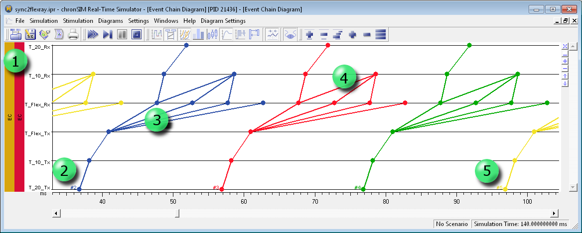
Figure 7.35: Event Chain Diagram #
Event Chain Graph Constraints#
The Tool-Suite reconstructs a graph by connecting consecutive steps
of common chain and instance number.
A step is connected to a chronological successor,
if the successors step number is greater or equal.
Also, a certain step may have multiple successors.
Thus consecutive steps 1 - 2 - 9 - 10 and 1 - 2 - 6 - 3 - 4
are both valid step sequences, while in the resulting graph of the latter
both steps 6 and 3 will be successors of step 2.
Occurrence of multiple successors leads to branching of the graph.
Figure 7.36: Event Chain Visibility Dialog #
If you have defined symbolic step names for an Event Chain, these will be shown as labels on the y-axis of the chain's diagram.
The start of an Event Chain instance graph is denoted with the instance number.
In case of more then one succeeding steps with identical step number, the chain instance graph will branch.
The predecessor of a step may be ambigous after branching.
Chain instance graph colors repeat after reaching the last defined chain instance color.
7.7.11 Histogram #
The histogram allows the analysis of the time distribution of an interrupt, of process or function execution times and in the most general case the latency of two arbitrary simulation events. [9]
Tip:
The evaluated simulation time range of histograms may be limited with the global time range filter
Tip:
As with evaluations of real-time requirements, individual measurements of the histogram distribution may be viewed in the process state diagram by using the context menu inside the histogram chart.
The following histogram shows the distributions of
the time span from one start of an interrupt service routine AsyncHandler on a processor CPU1 until the next start and
from one end until the next end.
In this example the interrupt has a nominal period of 100us
with an additional jitter using a normal (gaussian) distribution.
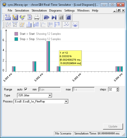
Figure 7.37: Histogram of Interrupt Jitter #
Elements of the histogram widget:
The legend explains which data is shown and how many samples have been evaluated
Each bar represents a data point
A tooltip follows the mouse and shows for each bar under the pointer the relative height and the interval it represents
When the auto option is checked the range of the histogram x-axis will be derived automatically.
Otherwise the user can manually enter the range and the number of intervals
This drop-down list contains the supported histogram types
Depending on the selected histogram type the dialog shows type specific options for that histogram
The evaluation of a simulation trace can take several minutes. A currently running evaluation can be stopped by pressing
The starts a new evaluation. This button will be enabled every time the simulation has generated new data or when basic selections have been changed
-
The allows exporting of the histogram as CSV or PNG.
-
The will add a diagram to the stack diagram view showing the time domain rollout of histogram values.
By selecting the menu entry → any number of histograms may be created. Initially the histograms are empty, they are filled only after selecting some options and pressing .
7.7.11.1 Available Histogram Types #
-
Bus Latency
This histogram shows the latency distribution of CAN messages for given CAN bus and CAN Id. events.
-
Event -> Event
This histogram shows the distribution of time spans between any two events.
-
Event Chains
This histogram evaluates the distribution of two steps of an event chain (see Section 6.2.13, “Event Chains”). To specify the steps and instances to be evaluated for the histogram see Section 6.6.12, “Event Chain Timing Requirement”.
Event(i) -> Event(j)
Events which are recorded by the use of the macro
EVENT1()[10] carry an integer parameter. This method allows the selection of two events and the definition how the parameteriof the first event has to correlate with the parameterjof the second event. The time span is only calculated for events where the relation matches.Idle Tme
This histogram shows the distribution of idle times for a given CPU core.
ISR Jitter
This is the example shown in Figure 7.37, “Histogram of Interrupt Jitter”. The time span between to starts and two ends of an interrupt service routine is calculated.
ISR Latency
This method calculates the statistical values of the delay between
occurrence of an interrupt and the execution start of the corresponding interrupt service routine,
between the interrupt occurrence and the end of the interrupt service routine, and
between the start and the end of the interrupt service routine.
OSEK Task Jitter
This will the show the characteristical jitter of a given OSEK Task by measuring the time difference of corresponding activation and execution events. This may not be possible in case of OSEK tasks which show a pattern of unrelated activation and execution.
OSEK Task Latency
Similarly to ISR Latency the latency of a given OSEK Task is calculated
Requirement
Shows the distribution of evaluations of a real-time-requirement
-
Value of Event(i)
This histogram shows the distribution of values recorded from simulating source code instrumented with the
EVENT1()macro.
The parametrization of most histogram types require the selection of two simulation events. By clicking an event the Object Selection dialog will be shown, which allows flexible filtering and selection from all the project's implicit and explicit (instrumented) simulation events.
7.7.12 Box Plot Diagram #
The Box Plot diagram gives an overview of all the simulated system's process response times. [11] For each process the response time minimum and maximum, the median and quartiles (4-quantile) are shown. The diagram window offers different options for sorting the processes by e.g. name, quantile or response time.
If chronVAL analysis has been run prior to the simulation,
the box plot will also visualize the results for best case and worst case response time results
from the realtime analysis (indicated by a green and red "^").
Since the realtime analysis is by definition more pessimistic then the simulation,
the results from simulation will always lie within the range of best and worst case
from the chronVAL analysis.
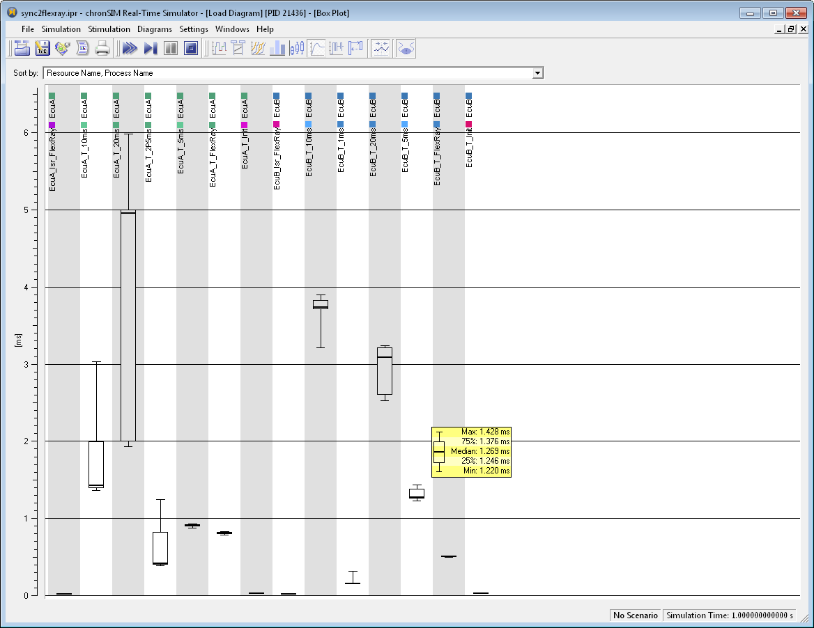
Figure 7.38: Box Plot Diagram of Process Response Times #
7.7.13 Load Diagram #
The load diagram displays the computational utilization of processing resources (microprocessors) and bandwidth utilization of communication resources (communication buses). The load of buses like CAN, Ethernet or FlexRay is derived the from sent packets. For each CPU and CPU core the load is shown as a stacked graph, with the loads of each process [12] shown with its process color. The diagrams of all CPU and bus resources are grouped along with each other in one window. See Section A.2, “Load Calculation” for details on the calculation of load values).
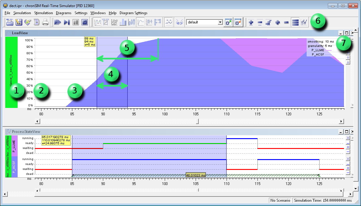
Figure 7.39: Load Diagram of a CPU with two tasks #
The items in the picture above denote the following items:
CPU Resource identifier
Resource utilization scale in percent
Utilization graph of the resource
The diagrams granularity interval (highlighted)
The diagrams smoothing interval
Button to adjust granularity and smoothing
Current granularity and smoothing value
7.7.13.1 Load Graph Grouping #
The Load Diagram allows to to collate a number of individual process loads to be shown as a single load graph. For this two special groups named Base Load and Rest Load may be shown at the bottom and the top of the load diagram. This is useful in case of an ECU with many processes and/or ISR's in order to
summarize the load of a group of associated processes or
deemphasize the load of a group of processes not of interest in order to raise attention to processes under consideration.
In order to define or modify a Base Load of Rest Load group use either → or → from the context menu.
The follwing figure shows the load diagrams of an ECU of the
AutosarMulticore.ipr example.
The first diagram just shows the original load graphs of all processes and ISRs
whereas in the second diagram the load of all ISRs is grouped as Base Load
and the load of the processes swcB and swcB
is summarized as Rest Load.
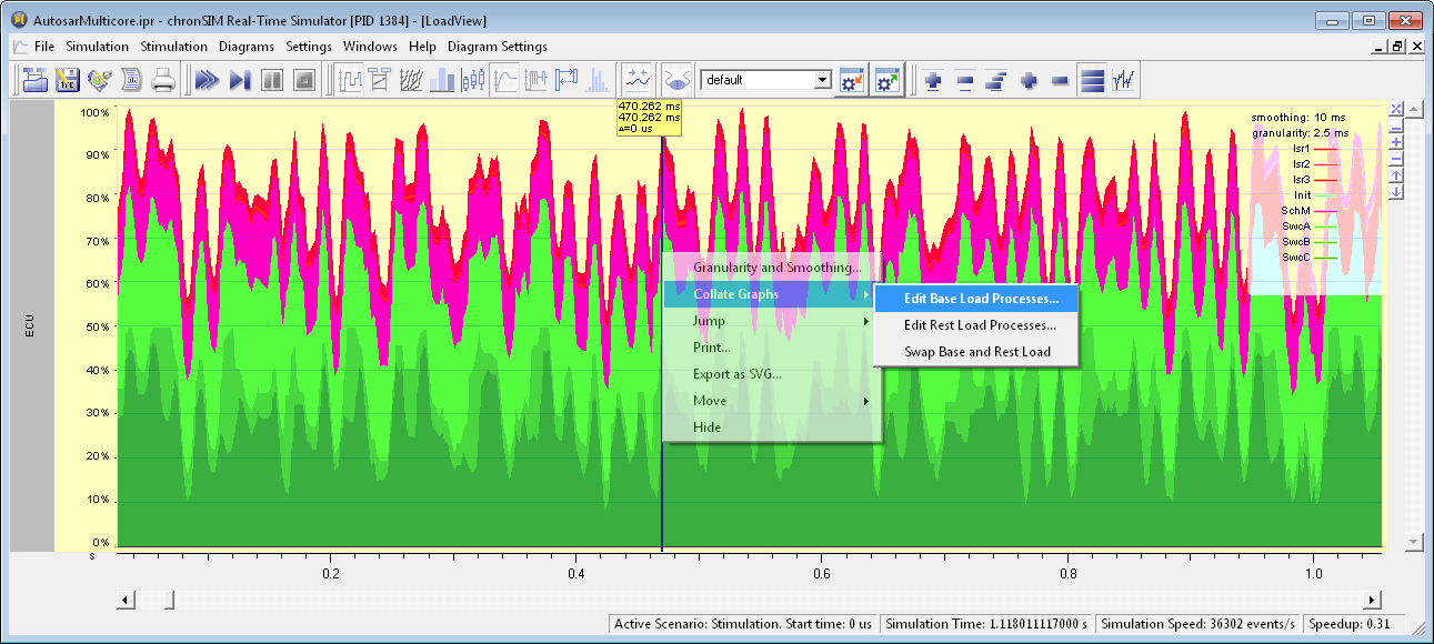
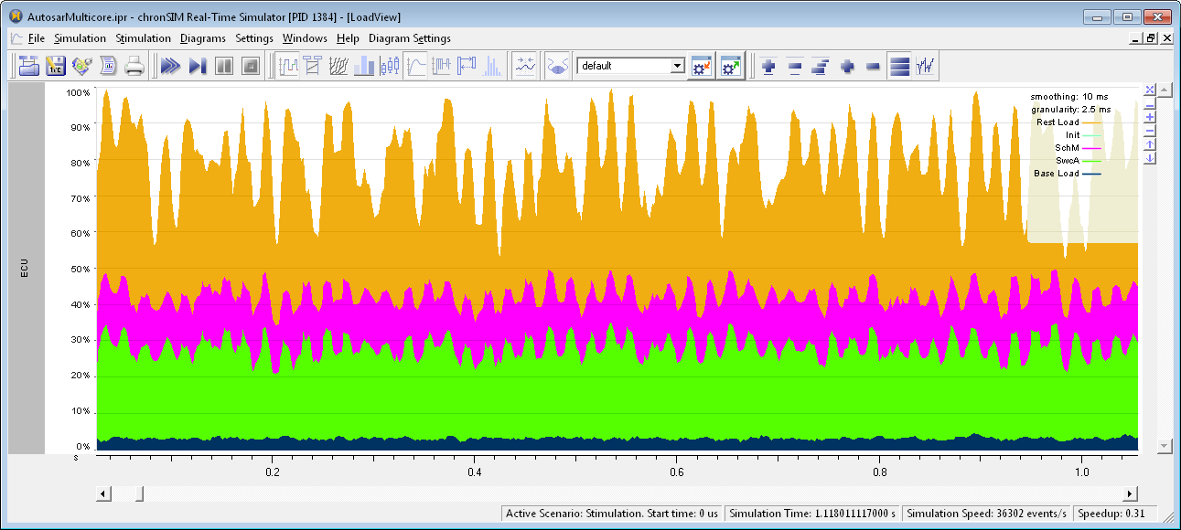
Figure 7.40: Collating Load Graphs #
7.7.13.2 Load Graph Granularity and Smoothing #
The load diagram offers additional settings affecting the visualization of data. These parameters can be altered via the menu.
Resource utilization data is aggregated as follows:
load mean values are calculated in equidistant granularity time intervals.
a smoothing filter is applied with the smoothing interval being a multiple of the granularity interval.
In case of the smoothing interval being longer then process execution times, at a given point of time more then one process will show a contribution to the resulting load of a processor core. See Section A.2, “Load Calculation” for details on load calculation of CPU and bus resources.
The Smoothing and granularity time intervals may be adjusted to your needs.
-
The granularity denotes the distance between two load calculation points. The granularity parameter allows you to compromise between load data precision and drawing speed. Smaller values increase the computation time for the calculation of load values (especially in case of a large diagram time range), whereas larger values result in a less precise graph. A sensible granularity value is below
1%of the diagram time range. The granularity may be be set to be calculated automatically by specifying an arbitrary periodic simulation event -
Smoothing defines an averaging interval which is applied to interpolated load values. E.g. with a smoothing interval of
1ms, each data point of the graph shows the arithmetic mean of CPU utilization of the time interval of1msbefore and up to that point in time. The smoothing parameter is specified as a number of averaging filter steps and therefore its value is always a multiple of the granularity time interval.
Figure 7.39, “Load Diagram of a CPU with two tasks” above clarifies the relation between granularity and smoothing.
In the example a Granularity interval of 5ms (item 4)
and a smoothing window of 10ms (item 5) is set.
At simulated time 85ms the first CPU becomes active
by process P_LLME changing from state waiting to running.
The first non-zero load value at 89ms evaluates to 40,
resulting from 4ms CPU activity inside the 10ms smoothing interval
before and up to 89ms.
After simulated time 110ms the
load of process P_LLME declines
to be replaced by load contribution of process P_ACSF
The shown load of the latter process never reaches 100%,
because its execution time is shorter then the averaging interval given by Smoothing.
Note:
The load graph linearily interpolates load data points by connecting adjacent data points. Thus when zooming the load diagram, the load graph will show non-zero load inside a granularity interval where the CPU becomes running. This effect may be avoided by increasing the granularity of load values (i.e. decreasing the granularity value).
7.7.13.3 Setting Granularity and Smoothing #
The granularity and smoothing parameters are adjusted with the
Granularity and Smoothing Dialog via
→ ,
with the corresponding diagrams
 toolbar button or from a load diagram's context menu.
In the latter case, the chosen settings will apply to the current load diagram, if you did not check the Apply to all diagrams option. In case of invocation via menu or toolbar, the settings will apply to all load diagrams.
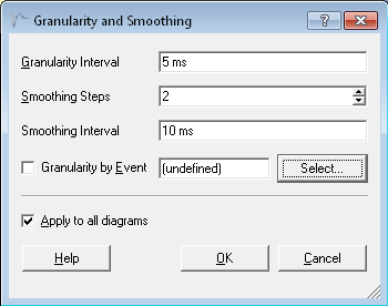
Figure 7.41: Granularity and Smoothing Dialog #
The Smoothing Interval results as the product of the Granularity Interval and the Smoothing Steps input fields. When editing the Smoothing Interval directly, the Granularity Interval will be adjusted accordingly leavine Smoothing Steps as is.
7.7.13.3.1 Granularity by Event #
With the Granularity by Event option you may choose the granularity to be automatically derived from the period of a simulation event, This may be e.g. the periodic activation of a process or ISR or any other simulation event. If is recommended to have run the simulation for at least two periods before activating this option. In this case the dialog will estimate the event period from current simulation trace data to give a preview of resulting value.
7.7.14 Stack Diagram #
The stack diagram displays the changes in stack usage of each task over the time. Each task is shown in a separate diagram. All tasks' stack diagrams are grouped together in one window.
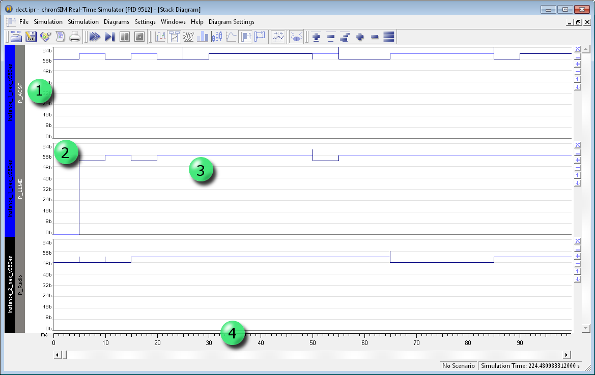
Figure 7.42: Stack Diagram of example dect.ipr #
The items in the picture above denote the following:
Task Identifier
Size of stacks in bytes
Current stack usage
Simulation time scale on the target
7.7.15 Event Diagrams #
The purpose of an Event Diagram is to visualize a simulation event over time. There are three types of Event Diagrams with different processing of the event value, e.g. for event rate calculation or event counting as described below.
The Event Diagrams are only availabe in the Stack Diagram Window. The following procedure demonstrates how to add different types of Event Diagrams:
Procedure 7.2: Adding Different Types of Event Diagrams #
Use → from the Tool-Suite application main window and select the
apollo11/apollo11_SIM.iprTool-Suite example project.Click the toolbar button.
Use the tool button to open the Stack Diagram window.
Select → → .
Result:The Object Selection dialog opens.
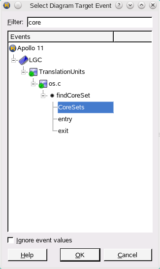
Figure 7.43: Select an event item #
In the Event Selection Dialog select the CoreSets event of function
findCoreSetin translation unitos.c. and confirm with .Tip:
For quick event lookup you may enter part of the event name in the Filter input field order to narrow the view on relevant items.
Result:A new Event Rate Diagram is added to the diagram window.
Repeat Step 4 with the → menu item, select the same CoreSets event for adding an Event Value Diagram.
Result:A new Event Value Diagram is added to the diagram window.
Repeat Step 4 with the → menu item, select the same CoreSets event for adding an Event Value Diagram.
Result:A new Event Counter Diagram is added to the diagram window.
After the procedure above the Stack Diagram window will show three Event Diagrams for the same system event as shown below. Each of the diagrams graphs will show the derivative of the diagram above.
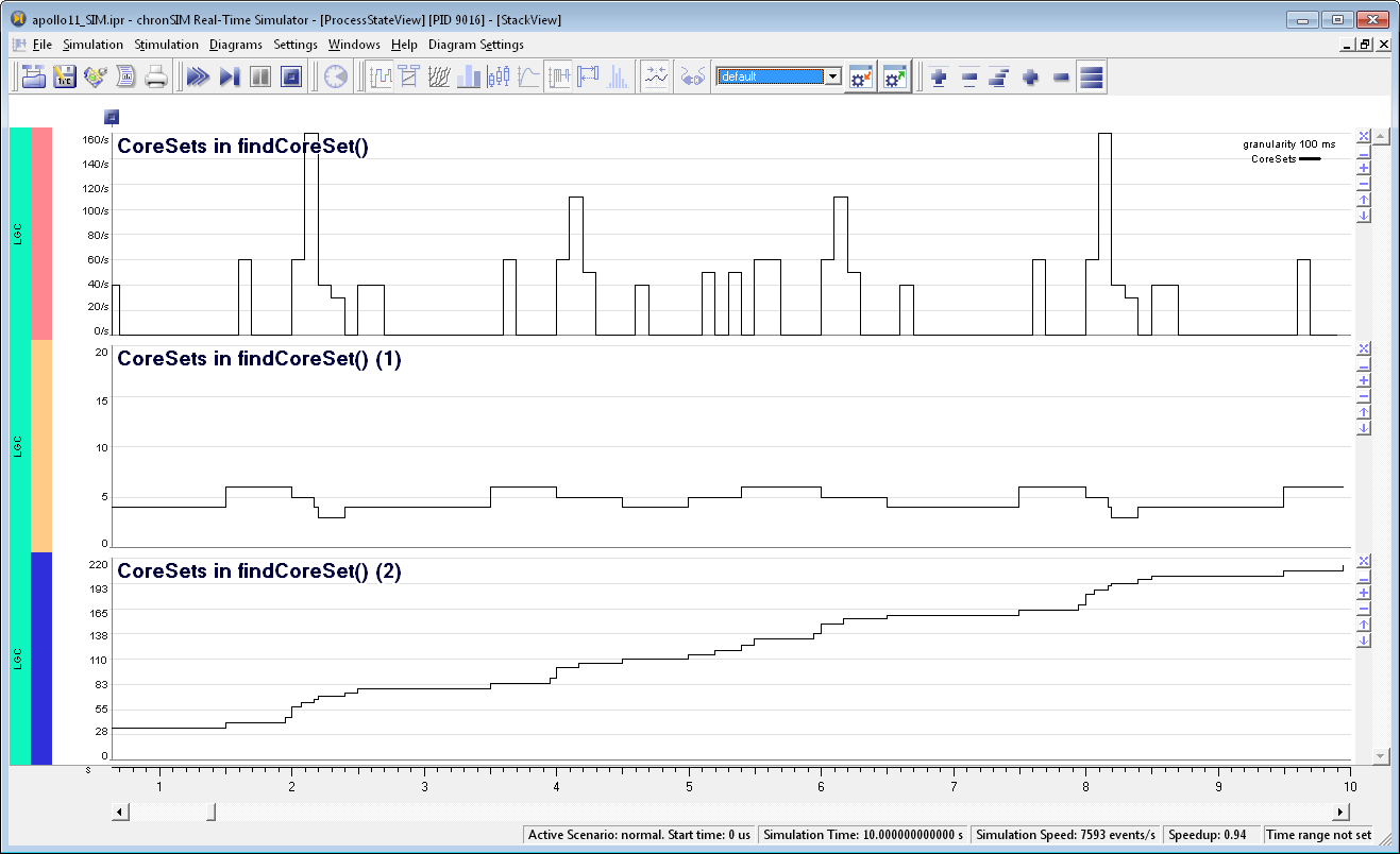
Figure 7.44: Adding and Removing an Event Diagram #
The three menu items have the following semantics
The adds a new diagram which visualizes the
valueparameter of source codeEVENT1()[13] instrumentation over time.The adds a diagram for visualizing the (monotonically increasing) count of any implicit or explict event.
The adds a diagram for visualizing the event rate of any implicit or explict event.
Tip:
As shown, you may add multiple types of event diagrams for the same event
While per process diagrams can only be hidden an event diagram may also be removed using from its context menu.
The Event Rate Diagram allows adjusting granularity and smooting like the load diagram.
7.7.16 Nesting Diagram #
The function nesting diagram shows each task's function calls and call nesting depth over time. The function nesting depths and function execution duration of all tasks are displayed together in one window.
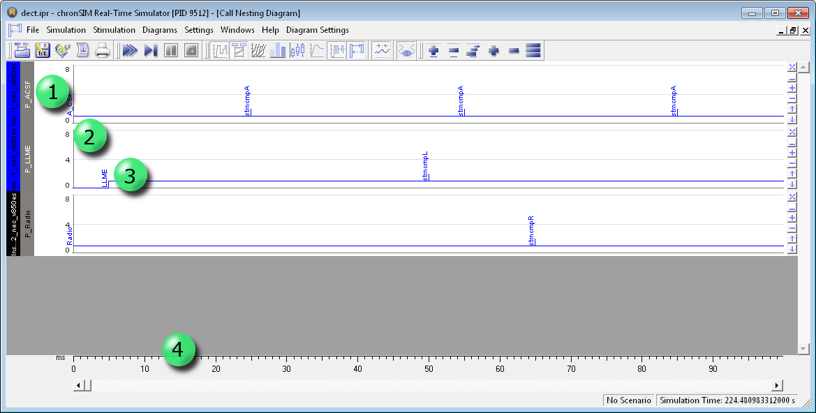
Figure 7.45: Nesting Diagram of Example dect.ipr #
The numbered items in the picture above denote the following:
Task Identifier
Call nesting depth scale
Current function nesting depth and function execution duration. An upward change symbolizes a function call, along with a character string denoting the called function's C name. A downwards change indicates a function returning to its caller.
Simulation time scale.
7.7.17 Console View #
A Console View is an instrument to visualize formatted messages from simlulated C code or data being transferred on ports of bus peripherals. It either
visualizes printouts from simulated C functions or
allows to inspect data from peripheral ports
The following screenshot shows a Console View
from the candemo.ipr project
in the examples/Can directory.
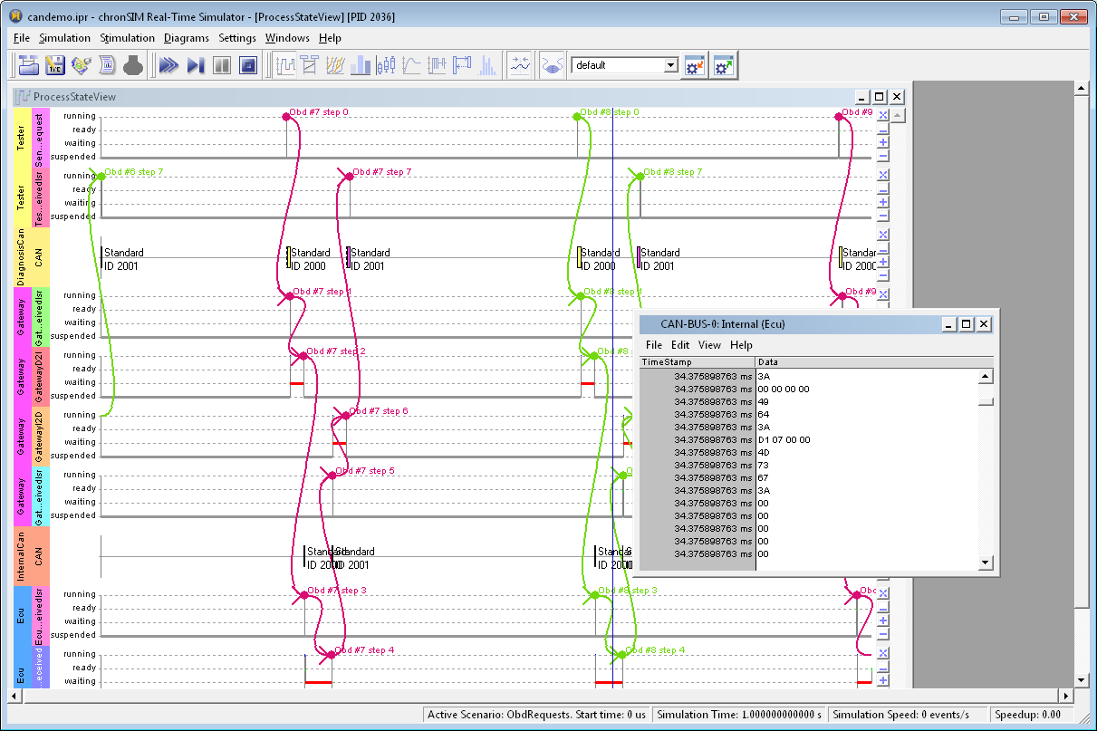
Figure 7.46: ConsoleView Example Can/candemo.ipr #
The data shown in the console view of may be formatted in either ASCII, hexadecimal or binary using the options of the console view menu. Output from different simuation data sources is shown in dedicated Console View windows.
7.7.17.1 Visualizing Console Printouts #
Using a Console View it is possible to log output
of all printf() function calls
from simulated C code for a certain CPU resource.
Since the concept of the ConsoleView is based on visualization of peripheral port data,
it is required to add a single console peripheral
to all CPUs for which printf() instrumentation shall be recorded
in the simulation trace file.
After that all console output on stdout and stderr
on that CPU will automatically be recorded as output of this console peripheral.
For each CPU with a console peripheral the simulator window will show two entries stdout: con and stderr: con in its → → .
Important:
The
printf()function provided by INCHRONCLib.h[14] only provides a subset of the standardized functionalilty. Flags, field width and precision parameters in theprintf()format string are currently not supported.The C++ output streams
cout,cerrare currently not supported by Console View.
Tip:
Alternatively, short state information from simulated C code may be also be visualized
in the sequence diagram
by instrumentation with the STATE(),
EVENT() and EVENT1() macro.
[15]
7.7.17.2 Visualizing Peripheral Data #
In general the Console View is an instrument to continuously visualize bulk data from peripheral ports. A dedicated Console View window is available for all ports of all peripherals of a system model. The corresponding menu items can be found under → → , like shown in the screenshot below.
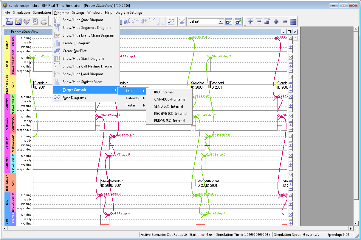
Figure 7.47: ConsoleView Example Can/candemo.ipr #
7.8 Saving and Loading Trace Files #
A simulation trace may be saved to a trace file for purpose of documentation. Saved trace files may also be loaded at any time into the Tool-Suite application again for analysis and inspection.
It is also possible to archive a simulation trace to a subversion repositoryfrom within the Tool-Suite as described in Section 12.5, “Version Control for Simulation Traces”.
7.8.1 Saving a Trace File #
Saving the simulation trace to file is done as follows:
Pause your current simulation by clicking
Select → .
Use the file save file dialog to select a target file with extensions ISF (INCHRON simulation file)
Saving long-running simulations of complex models may take several minutes. The progress of saving will be indicated by a progress bar.
After saving you can continue your simulation as usual.
7.8.2 Loading a Trace-File #
A previously saved simulation trace can be loaded from a file both from the project view as well as from the simulator window, no matter if a simulation is already running or not.
The Tool-Suite application allows you to load and view multiple trace files in parallel. Each trace file is displayed inside its own instance of the chronSIM Real-Time Simulator window.
In order to load a simulation trace use → from the menu.
The selected trace file will be opened in a separate viewer instance of the chronSIM Real-Time Simulator window.
The analysis and visual presentation of a loaded trace file is done the same way as with a running simulation.
7.8.3 Trace File Import or Export #
The INCHRON Tool-Suite comes with a wizard for importing custom trace file from CSV. This import feature is available from either the editor mode or simulation mode main window via → . This import feature is also part of the chronVIEW feature described in Section 3.2.5, “The Viewer Mode”.
Exporting of simulation traces is supported via command line tools, see Section B.4, “traceconv.exe”.
7.9 Export of Stimulation Scenarios #
The Tool-Suite allows the export and import of stimulation data used for a particular simulation run. Using comma separated values (CSV) as export format, it is possible to edit or process stimuli data with spreadsheet applications or other 3rd party tools.
7.9.1 Reproducibility of Random Stimulation #
The use of random stimuli generators prohibits successive simulation runs with identical stimulation. In this case in order to reproduce a simulation run with identical stimulation you have to
run the simulation
export the simulation runs stimulation data as CSV
switch to project mode by terminating the simulation mode and select the Module Stimulation in the Tool-Suite main window
create a CSV based stimulation scenario which imports the stimulation exported before.
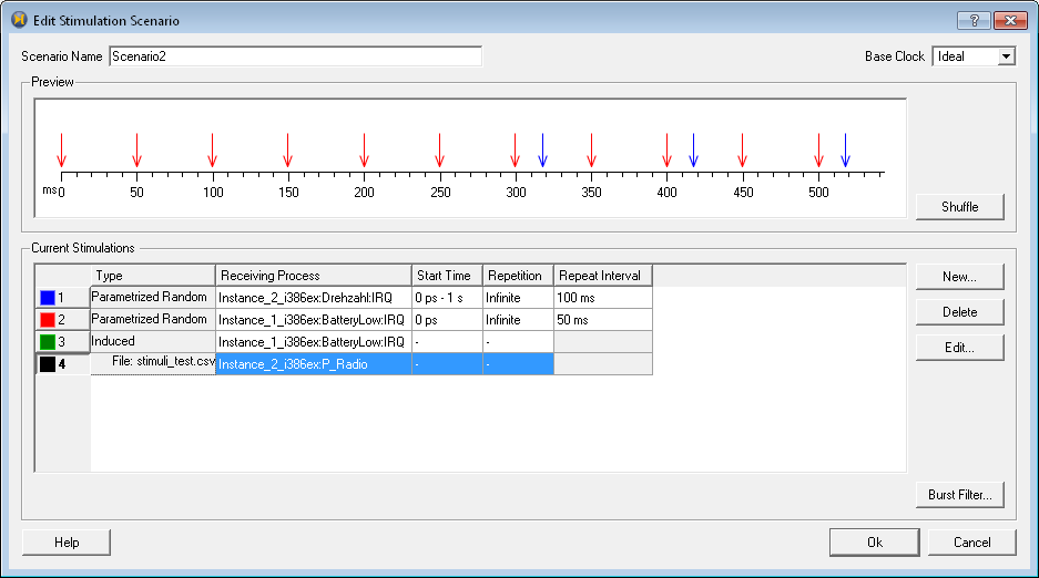
Figure 7.48: Scenario from CSV #
7.10 Reporting #
INCHRON Tool-Suite supports different types of export and report formats for simulation results for purpose of documentation and further processing.
The export of simulation diagrams (which is not subject of simulation reports) has already been described in Section 7.7.4.3, “Printing and Exporting Diagrams” and the export of the requirement evaluation summary has been described in and Section 7.6, “Real-Time Requirements”.
The dedicated report functionality of the INCHRON Tool-Suite allows the generation of a comprehensive summary of simulation results in different file formats. The default report format is HTML. The HTML report comprises separate sections for processing resources (CPUs) and communication resources (buses) and a summary of real-time requirement evaluations. These sections contain statistical information on resource utilization given as tables and additional histograms: For CPU resources process [16] (and optional function) execution time statistics is given and for communication resources statistics on sent messages for communication is given.
Regarding process statistics the report lists the following execution times for each simulated process:
- Response Time
Time from process activation to termination
- Gross Execution Time
Time from process start to termination
- Net Execution Time
CPU time (time spent in state running) between start and termination
Execution times are also given for all functions called by processes, while their definitions are not directly comparable with these of the corresponding process execution times:
- Response Time
Time from function entry to function exit
- Gross Execution Time
CPU time (time spent in state running) between function entry and function exit
- Net Execution Time
CPU time (time spent in state running) between function entry and function exit, excluding time spent in function calls
The appearance of the HTML report may be modified using a cascading stylesheet (CSS). Additionally, contents and structure of HTML reports may be customized as described in Section 7.10.2, “Report Customization”.
Beside HTML the report may be exported as CSV file [17] (without diagrams) or as XML file for further processing. [18] For the XML report format all reporting results are embedded into an IPR (INCHRON project) file.
The batch simulation command line tool provides options for the different types of report generation.
7.10.1 Report Configuration and Generation #
Per default the HTML (and CSV) report will contain sections for each processing and communication resource. The Report Configuration dialog allows configuration of
individual selection of processing and communication resources to be included,
granularity of process and function execution time and event requirement reporting and
histogram generation options
In order to configure and create a simulation report do as follows:
the
 report icon in the toolbar or use
→
.
report icon in the toolbar or use
→
.
The Report Configuration dialog will be shown.
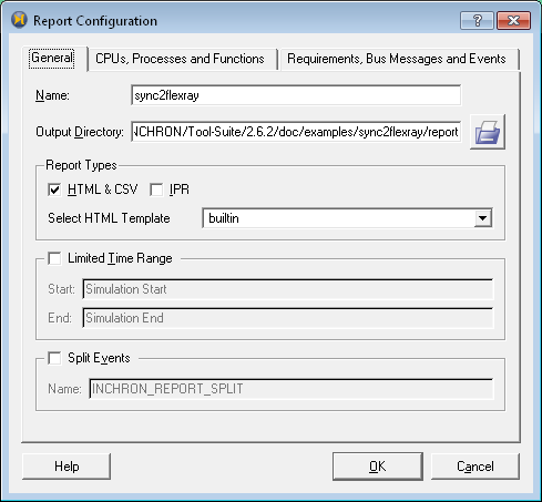
Figure 7.49: Report Configuration Dialog - General Options #
The dialog's General tab provides report destination and output format options, restriction of the report time range and optional automatical report splitting on occurance of a user defined event
The dialog's CPUs, Processes and Functions tab provides narrowing on the set of CPU resources and processes to be included and additional options for controlling the granularity of execution time reporting.
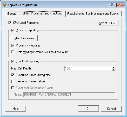
Figure 7.50: Report Configuration Dialog - CPU and Process Options #
The dialog's Requirements, Bus Messages and Events tab provides reporting options for Real-Time Requirement evaluations, events and peripheral buses (currently CAN and FlexRay).
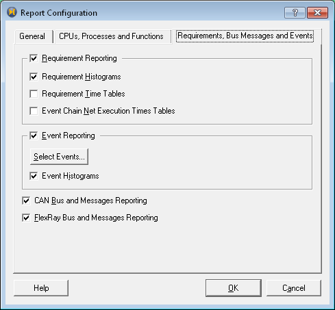
Figure 7.51: Report Configuration Dialog - Bus, Event and Requirement Options #
Adjust the report settings as needed and confirm with .
The report will be written to the selected output folder. Already existing files with same name will get overwritten. When finished the HTML report will be opened in your systems standard browser.
The following reporting options are available:
Category General
-
Name Report name to be shown in the title.
-
Output Directory destination folder for report
index.html, a style sheetstyle.cssand generated graphic files. -
Report Types Available formats are HTML, CSV and IPR.
-
Limited Time Range With this option reporting may be limited to a time range of the simulation trace (see also Section 7.7.1, “Time Range Filter”).
-
Split Events This option activates automatical splitting of the report at occurance of a user defined event using the
EVENT()macro (the default event is INCHRON_REPORT_SPLIT).
-
Category CPUs, Processes and Functions
-
CPU Load Reporting if checked, a table with statistical information about the systems CPUs will be included. With Select CPUS... individual CPUs and CPU cores may be selected.
-
Process Reporting if checked a table with statistical information about simulated processes and ISRs will be included. With Select Processes... individual processes may be (de)selected.
-
Waiting state End Execuction if checked, process waiting states of a process under the condition that the processes function stack is empty will be interpreted as begin of a suspend resume cycle. I.e. this will effect the statistics of the process by incrementing its execution count and yielding a new execution times measurement. This is especially useful for monitoring OSEK extended task Timing Budgets.
-
Function Reporting: this option determines whether and up to which depth function execution time statistics are included.
Tip:
In case of function recursion affected time intervals will be accounted more then once (depending on depth of recursion) for reported gross execution times of functions for which recursion occurs. This may even result in reported function gros execution times exceeding the simulation time.
Max. Call Depth defines the maximum call depth up to which functions shall be considered. A value of
1means that process or ISR entry functions are considered only.Execution Times Tables if checked function gross and net execution times will be listed as table.
Execution Times Histograms if checked function gross and net execution times histograms will be included.
-
-
Category Requirements, Bus Messages and Events
-
Requirement Reporting if checked a Requirements report section will be included. A table reports evaluation statistics of the projects realtime requirements including histograms of individual evaluations for timing requirements.
-
Requirement Time Tables If checked, the summary of requirement evaluations will include individual evaluation times of timing requirements. In the HTML report up to
100entries will be shown, when clicking the requirement evaluation histogram. -
Event Chain Net Execution Time Tables if checked the report will include execution time tables for Event Chain.
-
Event Reporting This option allows to include statistics for
EVENT1()instrumentation. The Event Histograms enables the generation of histograms of the event value distributions -
FlexRay Bus and Messages Reporting if checked detailed information about FlexRay buses and dynamic segment slots utilization will be included.
-
7.10.2 Report Customization #
The HTML report uses a cascading style sheet (CSS) for several formatting options.
For customization, the default style.css in the output folder may be replaced or modified.
Beside formatting via CSS and selecting report output options in the report configuration dialog,
the structure of HTML reports may be customized by creating a custom report template.
The built-in report template used by default is equivalent to the default template defined by the
TPL files in the
templates/html-sim-report/default subdirectory
of the INCHRON Tool-Suite installation directory.
You may customize the default TPL files
or even create and modify copies of the
templates/html-sim-report/default
directory, which will in turn appear in the Select HTML Template
combobox of the report configuration dialog of the simulation window.
[7] Since Release 2.6.2. Note: These events do not occur for ISRs and OSEK basic tasks
since these have no task state wait
[8] The '.' (dot) in a regular expression is a wildcard for 'any character',
while the '.' (asterisk) modifier means 'any number of occurrences of the preceding expression'.
Expressions enclosed by '[]' define an alphabet for matching a single character
[9] See Section 7.7.12, “Box Plot Diagram” for a specific view on process response times statistics.
[10] See Reference Manual of Macros and Functions which is available via the Tool-Suite's help menu.
[11] Detailed distributions of process response times and more general system latencies may be obtained using the Tool-Suite histograms
[12] with the exception of idle tasks).
[13] See Reference Manual of Macros and Functions which is available via the Tool-Suite's help menu.
[14] See Reference Manual of Macros and Functions which is available via the Tool-Suite's help menu.
[15] See Reference Manual of Macros and Functions which is available via the Tool-Suite's help menu.
[16] with the exception of idle tasks).
[17] Currently CSV output is implicitly activated with the HTML export option.
[18] Beyond that, simulated execution times may be exported as C file in order to be used as a base for a statistical task model. This e.g. facilitates the creation of a task model from an imported 3rd party trace file.
8 Validation #
The following explanations are related to an example INCHRON project which is part of the distribution and which can be loaded with → .
This section will guide you through the steps in using the chronVAL validation. Validation steps comprise
the start of chronVAL validation
the visualization of validation results
8.1 The Validation Concept #
By starting chronVAL the validation relevant parts of the system model are evaluated for a real-time analysis. The results are presented in two separate windows.
The chronVAL result windows use a different color scheme for easy distinction from chronSIM related windows.
Tip:
The chronVAL windows don't have to be closed in order to perform another validation, facilitating comparison of more then one chronVAL validation. Validation runs can be identified by a timestamp in the caption of the chronVAL windows.
8.2 Example of Task Interference on a Preemptive Task Model #
This additional example demonstrates how to use the chronVAL tool to perform schedulability analysis of a simple task set using a fixed priority preemptive scheduler.
-
Open the example project
chronVal\FPPS\fpps.ipr.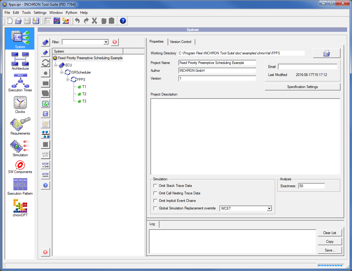
Figure 8.1: INCHRON Tool-Suite Window With chronVAL Task Interference Example #
-
A task set with three independent period tasks, as shown in table Table 8.1, “Modeled Example Task Set” is modeled using the System, Requirements and Stimulation module of the INCHRON Tool-Suite .
Table 8.1: Modeled Example Task Set #
Task
Computation
Time (ms)
Period (ms)
Deadline (ms)
T1
20
70
50
T2
20
80
80
T3
35
200
100
The tasks belonging to the task set, their priorities and the type of scheduler are modeled using the System module as shown below.
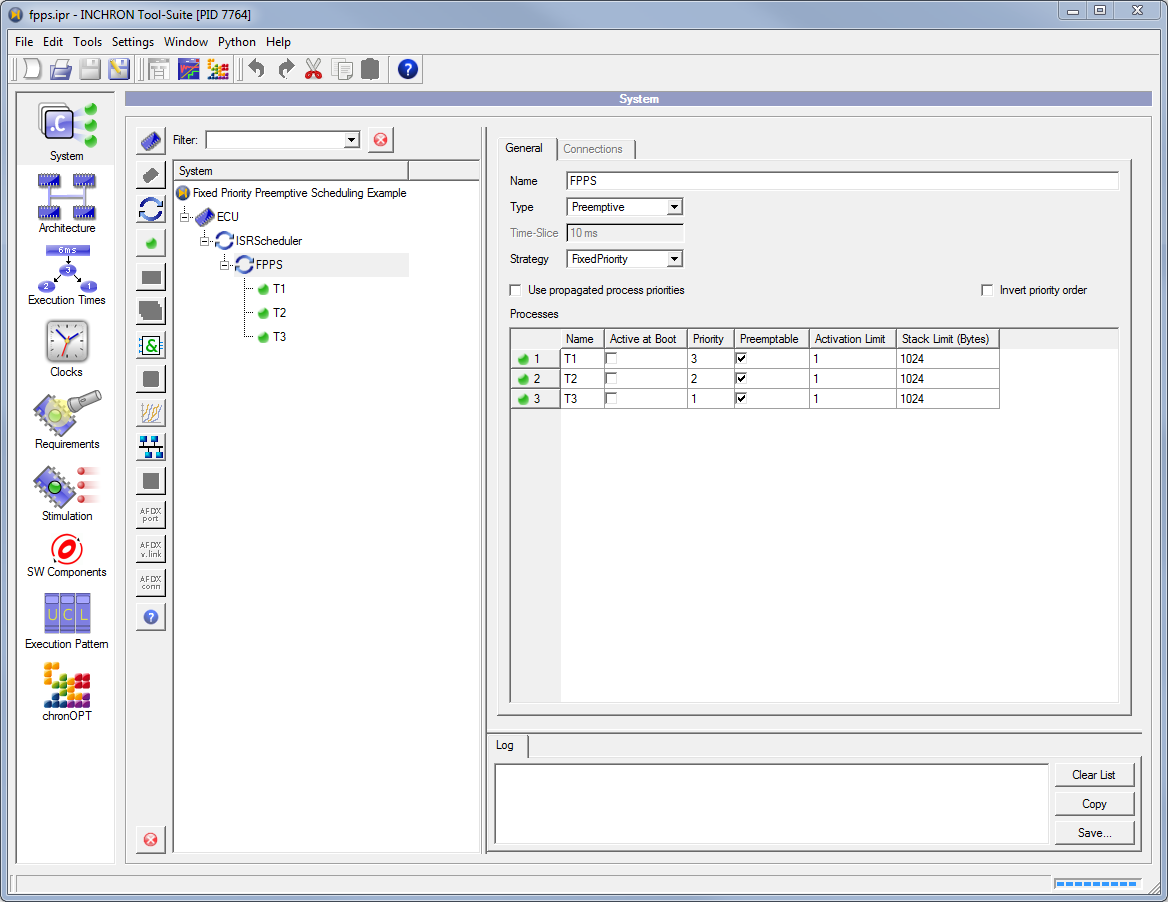
Figure 8.2: System Module Window With chronVAL Task Interference Example #
The deadlines of the tasks are modeled using the Requirements module as shown below.
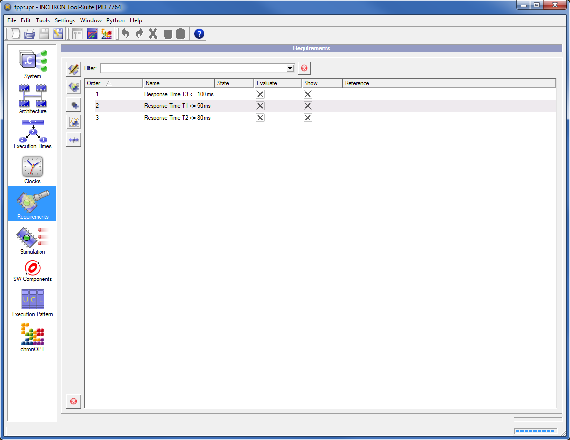
Figure 8.3: Requirements Module Window With chronVAL Task Interference Example #
The periodic activations of the tasks are modeled using the Stimulation module as shown below.
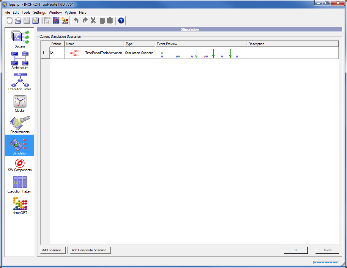
Figure 8.4: Stimulation Module Window With chronVAL Task Interference Example #
-
Start the analysis with the
analysis button or with
→
.
This initiates two chronVAL validation results window: Event Spectrum Viewer and Response Time Composition
-
Pull the Response Time Composition window to the front.
The Response Time Composition window shows for each task the its Deadline, its Worst Case Response time (WCRT) and the Best Case Reponse time (BCRT) (Figure 8.5, “Response Time Composition Window for chronVAL Task Interference Example”) in two bars (with differentation of task states for the WCRT case). Due to a WCRT of
115 msthe task T3 misses its deadline of100 ms. This is indicated by highlighing of the Deadline bar in red (above the WCRT bar).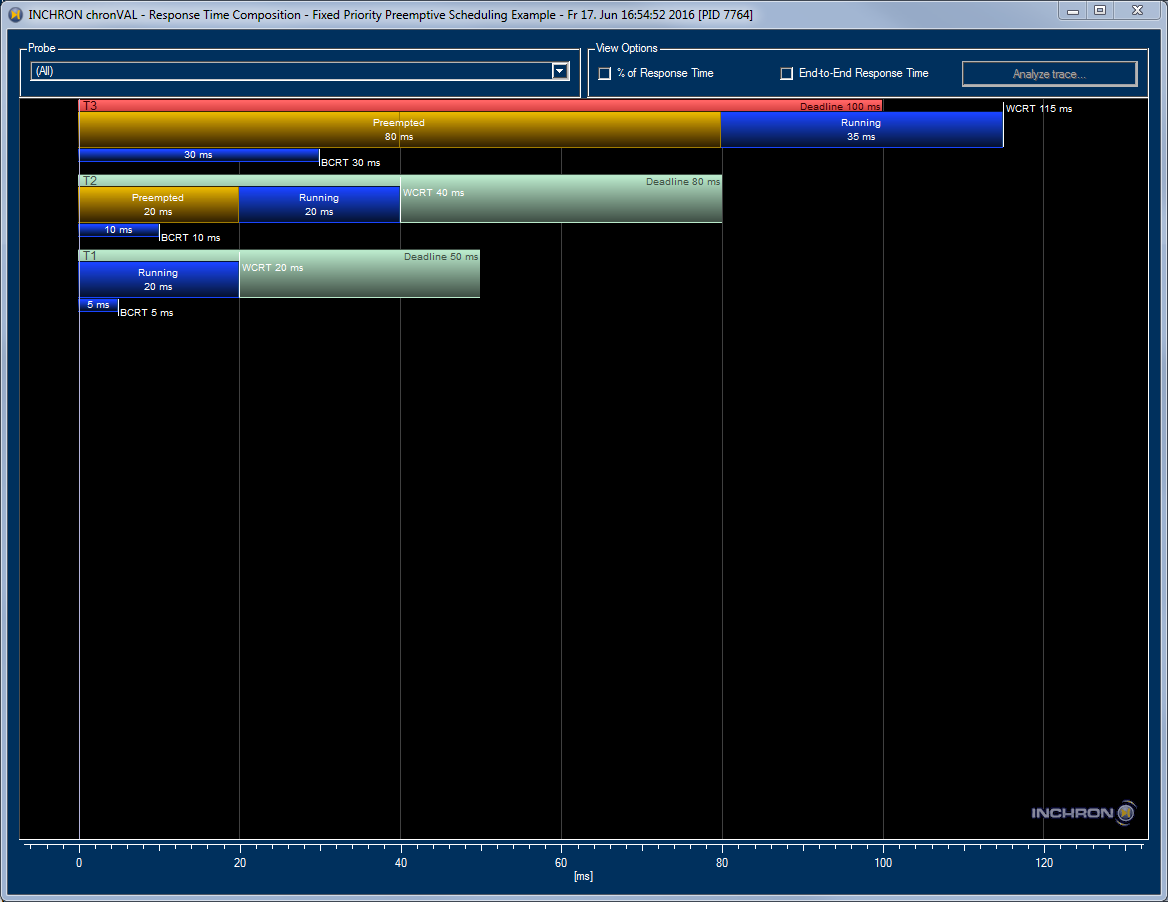
Figure 8.5: Response Time Composition Window for chronVAL Task Interference Example #
-
Select task T3 in the Probe drop-down list at the left top of the Response Time composition window.
In both Response Time Composition diagrams above (for all tasks) and below (for task T3) one can see that the worst case response time of the task T3 comprises two components (Figure 8.6, “Response Time Composition Window of Task T3”): The execution time (35 ms) of the task itself and the preemption time (80 ms) which equals the time for which task T3 is prevented from executing by higher priority tasks. The Response Time Composition additonally shows the composition of the task T3 preemption time which is composed of preemptions of 40 ms from both tasks T1 and T2.
Tip:
In order to further inspect task activations which are causing the worst case response time of task T3, you may click the Analyze trace... button in the View Options group box which will show a simulation trace for that scenario in a separate window.
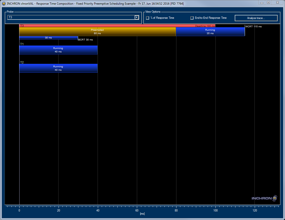
Figure 8.6: Response Time Composition Window of Task T3 #
-
Now pull the Event Spectrum Viewer window to the front. Again select process T3, this time from the top left Probe Selection list. Then check the Max + from Computation Time options and Min - from Available Capacity options as shown in Figure 8.7, “Event Spectrum Diagram for Task T3” .
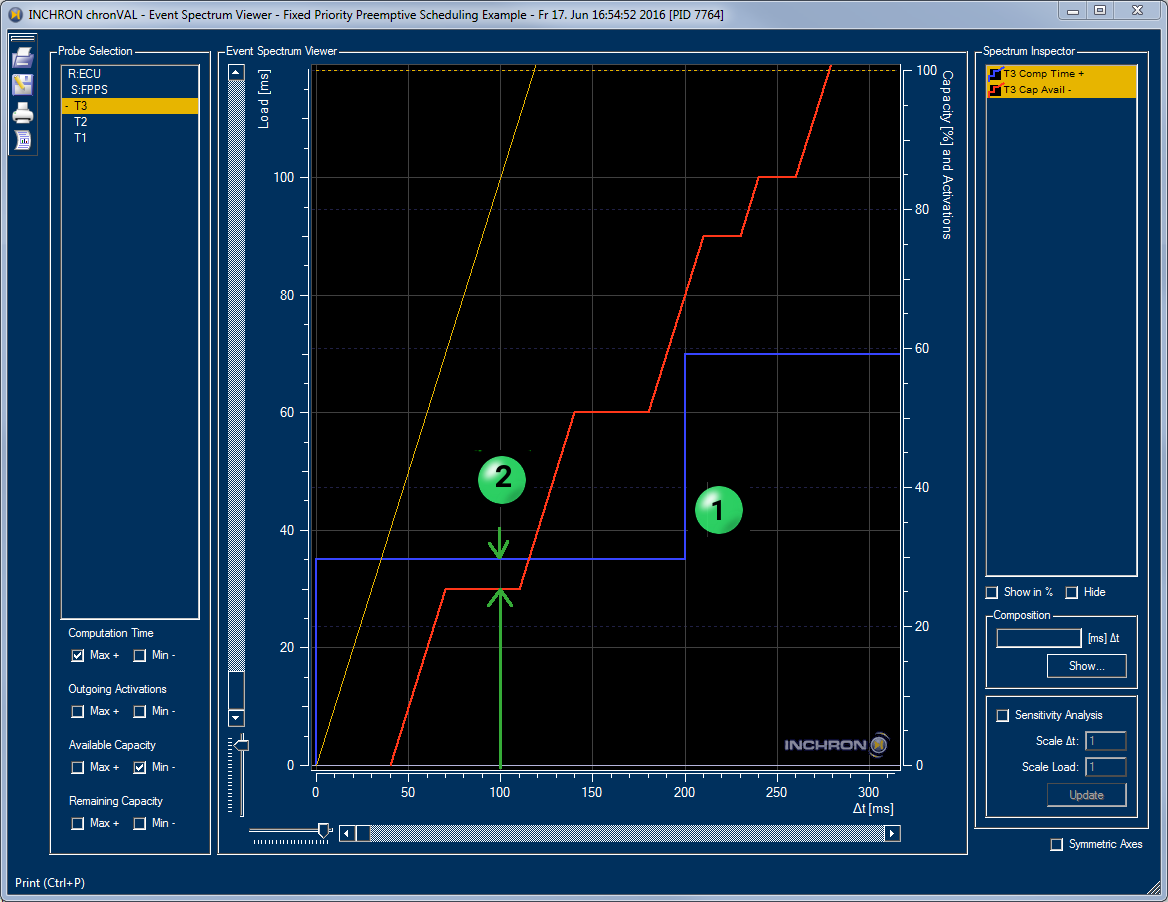
Figure 8.7: Event Spectrum Diagram for Task T3 #
The Event Spectrum Diagram for Task T3 above allows comparison of requested computation time and available capacity for any time interval. One can observe that for intervals of
100msthe blue graph shows that the maximum computation time request by process T3 for any interval is 35 ms (which applies to any interval up to 200ms).
However the minimum available processing time of task T3 in that interval is 30 ms as indicated by the red graph.
This implies that there exists an interval of 100 ms where task T3 cannot complete its execution. Hence task T3 with a periodic activation of 200 ms can miss its deadline of 100ms.
8.3 Example of Analyzing a Distributed System #
Performing the following steps will give you a quick overview on chronVAL validation:
Open the example project
chronVal\distributed\distributed.ipr.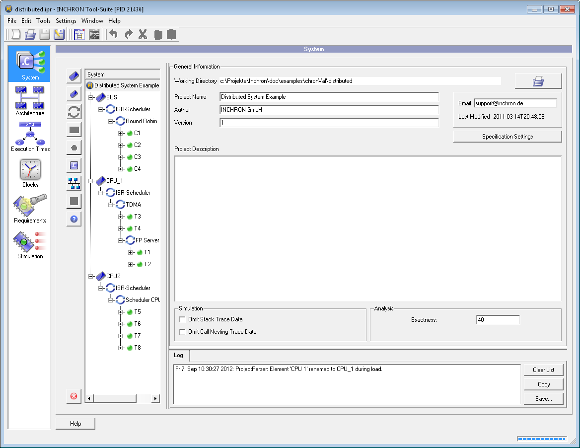
Figure 8.8: INCHRON Tool-Suite Window With chronVAL Example #
Start the analysis with the
analysis button or with
→ .Two validation result windows appear
Figure 8.9: chronVAL Analysis Result Windows #
Pull the Response Time Composition window to the front.
The window shows an overview of all task response times
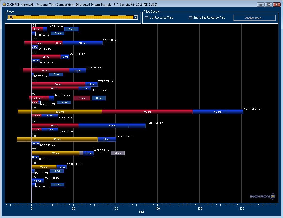
Figure 8.10: Response Time Overview #
In the probe drop-down list at the left top select the task T7.
The response time view shows three worst-case response-time bars. The first of these visualizes the worst-case response-time composition of process T7. Its response time of
74mscomprises12msfrom execution of T7 itself plus57msdue to preemption by processes T6 and T5 with higher priority and5msdefined blocking time, see Section 6.2.10.1, “Process Properties”.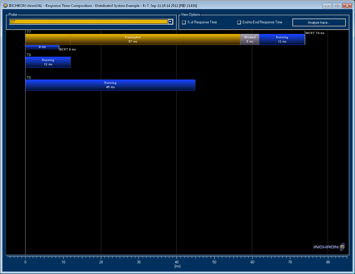
Figure 8.11: Response Time of Process T7 #
-
Now pull the Event Spectrum Viewer window to the front. Again select process T7 this time from the top left Probe Selection list-view
Select the option below the Remaining Capacity label.
The viewer shows the worst-case minimum remaining CPU time left over after executing process T7 for processes with a lower priority than process T7. The graph shows the remaining CPU time as a function of time intervals. For each interval length the minimum remaining capacity for all possible starting times of the interval is summarized to one minimum value by the analysis.
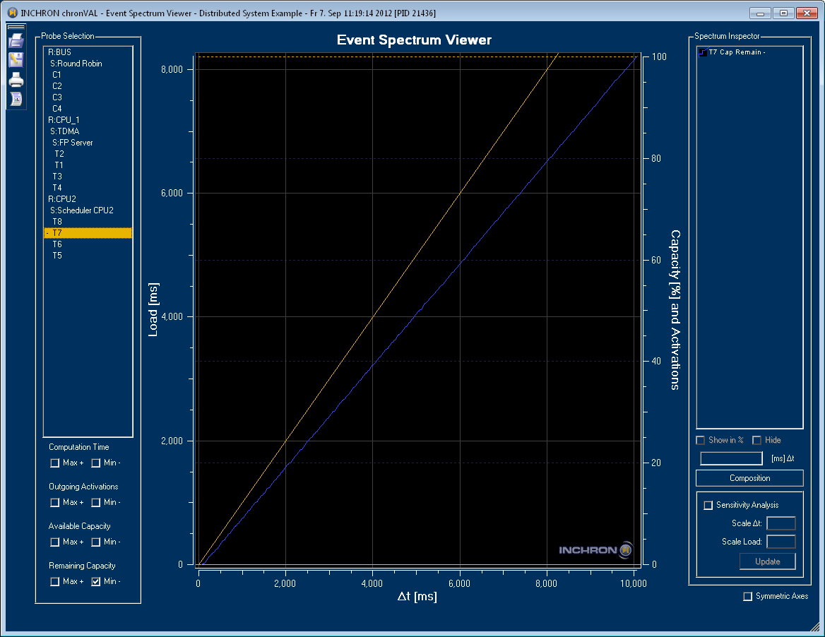
Figure 8.12: Remaining Capacity as Interval Diagram #
Now select the T7 Cap Remain entry from the Spectrum Inspector list-view at the right top and then check the option in the middle of the right side.
The graph of the minimum remaining capacity for T7 is now shown as percentage of the CPUs totally available capacity. Again the graph is over time intervals. For any interval below
100 msprocess T7 leaves now remaining CPU time. For longer intervals the remaining capacity is increasing up to its maximum at about80%(as shown at the right end of the graph).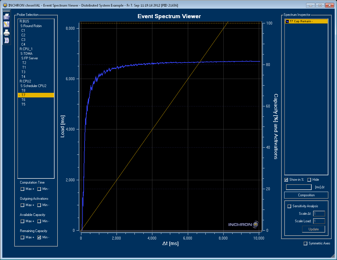
Figure 8.13: Relative Remaining Capacity Diagram #
8.3.1 Event Spectrum Visualization #
The INCHRON Tool-Suite validation is based on the chronVAL event spectra and the analysis of their interval diagram which are visualized by the Event Spectrum Viewer. (see Figure 8.14, “Event Spectrum Visualization”).
For this purpose the Event Spectrum Viewer provides several options for tailoring the event spectrum to the system to be analyzed.
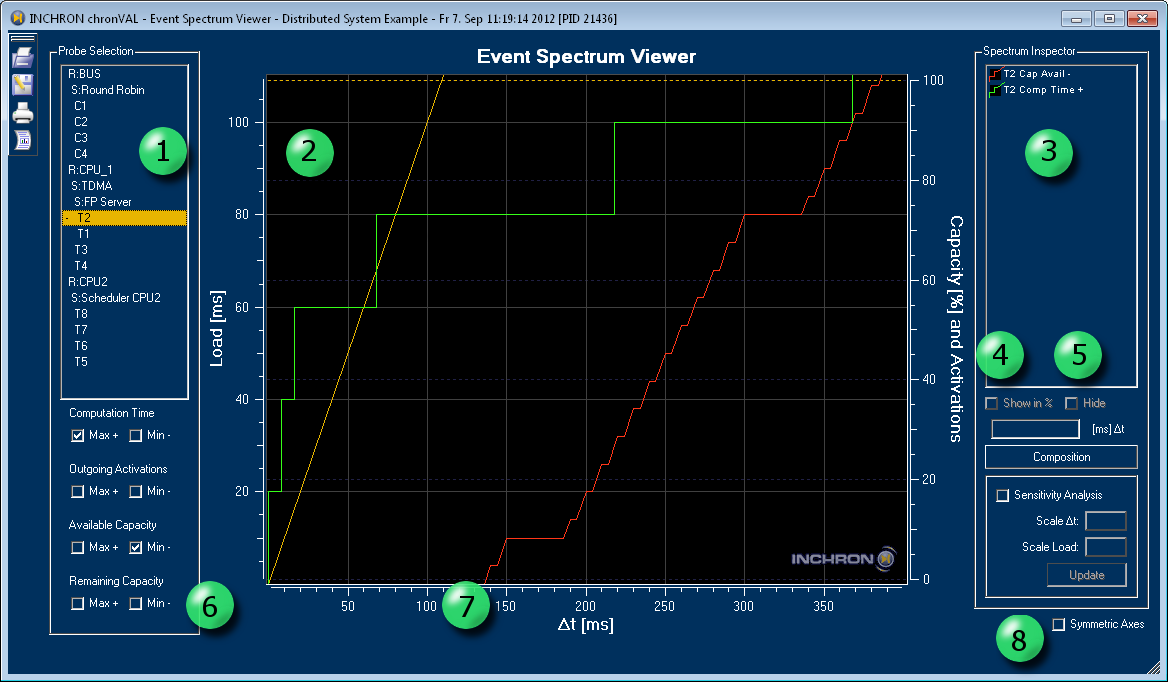
Figure 8.14: Event Spectrum Visualization #
The components of the Event Spectrum Viewer are
A list of processes and schedulers of the system
The drawing area for the event spectra
The drawing area always shows a bisecting line which represent the line of
100%load.The list of shown event spectra
A checkbox for toggling relative capacity axis
A checkbox for temporary hiding of event spectra
Max + and Min - checkboxes for toggling different process spectra described below. The state of these checkboxes is not global but instead each of the processes (1) has its own set of active spectra.
The time interval axis
A checkbox for toggling symmetric x- and y-axes.
For each process the following spectra are available:
Computation Time - the maximum computation time requested by the process for each time interval
Computation Time - the minimum computation time requested by the process for each time interval
Outgoing Activations - the maximum number of possible activations of subsequent processes for each time interval
Outgoing Activations the minimum number of possible activations of subsequent processes for each time interval
Available Capacity the maximum available processing time for the process for each time interval (best case)
Available Capacity the minimum available processing time for the process for each time interval (worst case)
Remaining Capacity the maximum processing time this process leaves for lower priority processes for each time interval (best case))
Remaining Capacity the minimum processing time this process leaves for lower priority processes (worst case)
Multiple process spectra may be activated or deactivated at once by first selecting multiple processes (1) and then toggling different spectra (6). In order to select multiple processes from the list (1) either the Shift or the Ctrl key have to be pressed while a process in the list.
The graph colors are assigned automatically. The list of spectra (3) shows short names of the spectra and their graph color like in a legend. The switching between relative and absolute y axis of individual spectra is possible by selecting one or several items (again either with the Shift or the Ctrl key) in the list of spectra (3) and then (4).
8.3.1.1 Scaling #
Initially the drawing area is scaled so that a sufficient number of steps is shown for each spectrum.
The scaling of the graph drawing area (2) may be zoomed as follows:
Move the mouse one edge to one edge of the area to be detailed and to start dragging.
Move the mouse to the opposite edge of the area to be detailed.
A rectangular area will be highlighted. If not the maximum zoom factor is already reached.
Release the mouse button
The drawing area zooms to the selected rectangular area.
With a with the right mouse button the original default scaling will be restored.
8.3.2 The Response Time Window #
The Response Time Composition window shows the worst case response times for a selected process. This is shown as a bar which is divided into the following main parts:
Preempted - cumulative time of preemption by processes of higher priority. In case of more than one preemption this part will be subdivided in parts of corresponding length .
Blocked - blocking time (e.g. non-available CPU in case of TDMA scheduling, see Section 6.2.10.1, “Process Properties”)
Running - own execution time
The selection of processes to be shown and the options for switching to relative y axis or end-to-end response time allow for purposeful analysis of the deciding factors for the real-time capability of the system under consideration.
The elements of the Response Time Composition window comprise
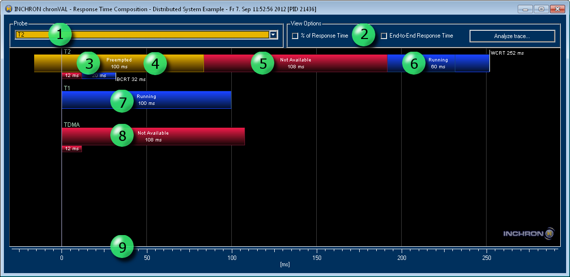
Figure 8.15: Process T2 Response Time #
List for process selection
Composition view options
best case response time
preempted portion of the worst case response time
portion of the worst case response time in which processor is not available (e.g. due to non-availability in case of TDMA scheduling)
running portion of worst case response time
amount of execution time of another process (T2) preempting the selected process (T2) (usually due to higher priority)
amount of execution time for which the processor is not available for a scheduler the selected process (T2) due to the scheduler (TDMA) (e.g. the amount of time slots which are not allocated to T2 within the response time of T2)
time axis
Manual scaling of the composition view is possible in the same way as of the Event Spectrum Viewer
Per default the view will be scaled to the maximum response times of all selected processes
8.3.2.1 Response Time History #
Usually a response time composition bar starts at 0 ms.
This is the case when the worst-case response time of a process or
message can be reached starting with an idle system.
In some cases the worst-case response-time gets an additional delay
by activations occurring before the activation of the process
leading to the worst-case response-time.
This can be either previous activations of the process itself
or of other processes.
In these cases the process suffers an additional delay
due to remaining load on the processor at the time of its activation.
In these cases the response time will appear with a negative portion as shown in Figure 8.15, “Process T2 Response Time”.
This case may be understood by coming back to the Event Spectrum Viewer. For this select the Computation Time Max + and the Available Capacity Min - spectra of process T2 like shown in Figure 8.16, “Illustration of Response Time of Process T2 in the Event Spectrum”.
The graph (1) shows the CPU time of process T2
for the worst case stimulation which reads as follows:
In a time interval of 100 ms (x-axis), the process
requires 80 ms CPU time in total for all of its
activations within this interval
(y value at x = 100 ms).
Graph (2) shows the minimum capacity (available CPU time) available for T2 in the worst case. The execution of a process can be finished in the smallest interval in which its required computation time is available as capacity. Hence the longest horizontal distance (3) between graph (1) and graph (2) is the worst case response time of T2.
The fact that the time interval (4) to be considered is bigger than the worst case response time of T2 is indicated in the Response Time Composition diagram by a response time with a negative portion of according magnitude.
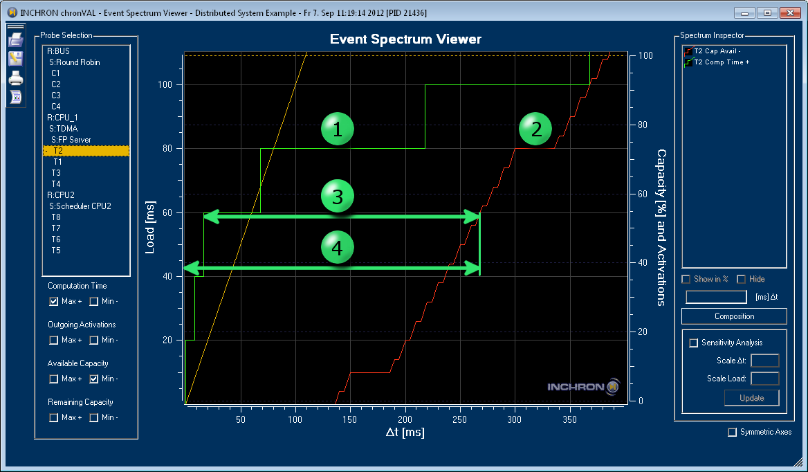
Figure 8.16: Illustration of Response Time of Process T2 in the Event Spectrum #
9 Optimization #
The chronOPT part of the INCHRON Tool-Suite provides a framework for optimization of an INCHRON system model regarding its real-time behavior. The objectives for expected real-time behavior for this purpose may be described by Real-Time Requirements.
The chronOPT functionality is integrated into the Tool-Suite as one of its main UI modules. Selecting the chronOPT main module will show the chronOPT configuration options. Configuring an optimization requires
the definition of optimization goals as objectives and
specifying the model's free parameters as Degree of Freedom.
Additionally, global settings, like global parameters of the search heuristics, different Halt Criteria and the objectives evaluation method (either chronSIM simulation or chronVAL validation) may be changed on the Parameters tab. The single available Search Method just named chronOPT is implemented as a tabu search, see Section 9.4, “Optimization Algorithm” for details. Additional search methods may be added by means of an extension mechanism.
9.1 Introductory Examples #
The INCHRON Tool-Suite distribution comes with two introductory optimization projects:
doc/examples/chronOPT/PrioTest.iprThis example is a quite simple optimization of both task priorities and core mappings in order to minimize response times of four specific tasks. A walkthrough of the example is given in the following sections.
doc/examples/chronOPT/chronOPT_2_Cores_and_25_Tasks.iprThis example like the one above adjusts both priority and core mapping of the project's tasks. The difference to the previous example is the increased dimension of the search space due to the number of 25 tasks and that the optimization goal is given by a greater number of partially conflicting objectives of different types, in particular for minimizing
the latency of two event chains,
task response times and
average load of the CPU cores.
In order to start with the PrioTest chronOPT example project select
→
and open the doc/examples/chronOPT/PrioTest.ipr example.
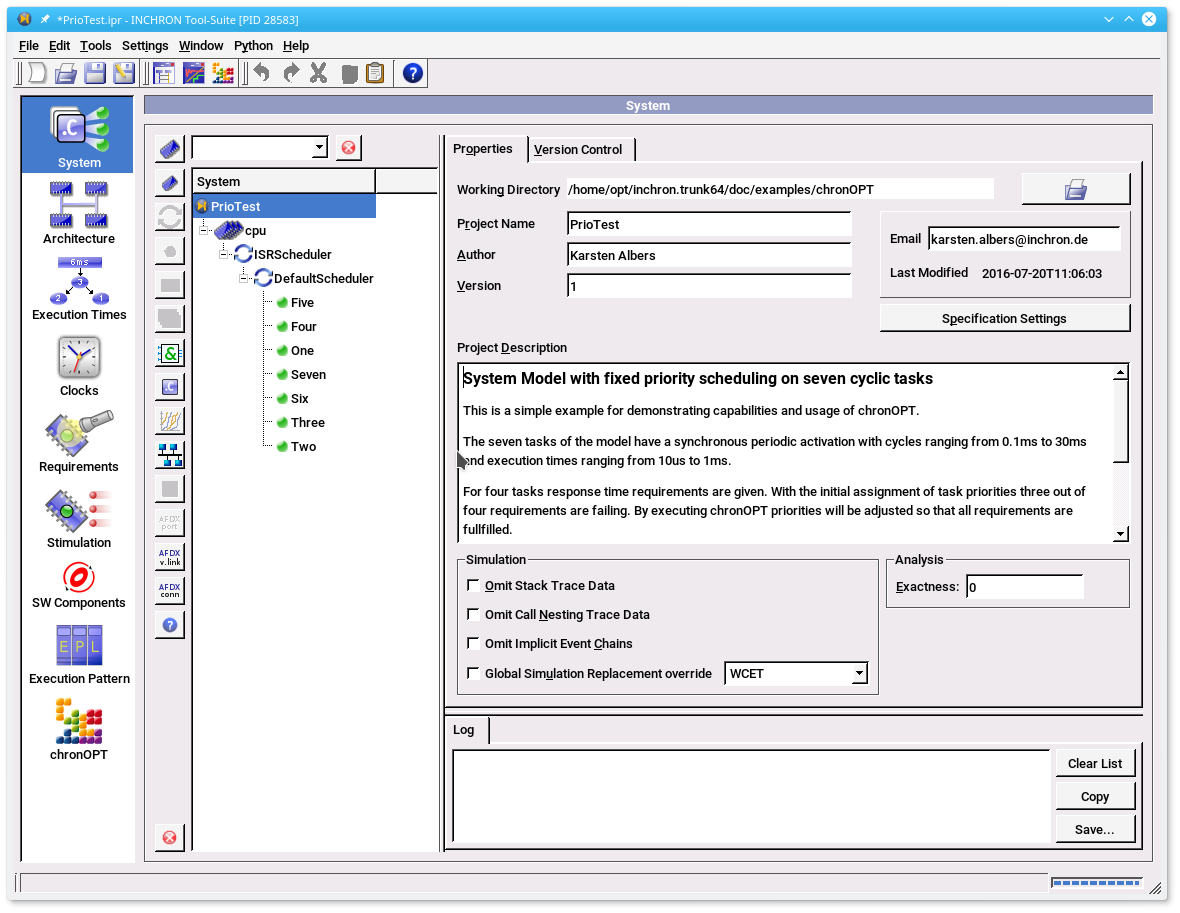
Figure 9.1: System Model of chronOPT example PrioTest.ipr #
Project Characteristics and Requirements#
The PrioTest.ipr is a system model
comprising seven tasks with synchronized periodic activation
with cycles ranging from 0.1 ms to 30 ms and execution times ranging from 10 us to 1 ms.
For the first four tasks response time requirements are given with limits ranging from 0.5 ms to 5 ms. With the initial assignment of task priorities three out of four of these real-time requirements do fail, which can be checked by running either chronSIM simulation of chronVAL validation on the project.
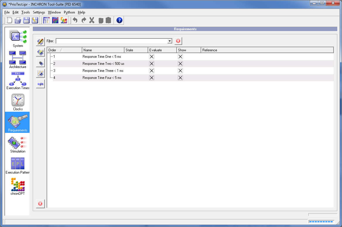
Figure 9.2: Real-Time Requirements for chronOPT example PrioTest.ipr #
Selecting the chronOPT UI module will show the Parameters tab which allows changing global parameters of the optimization like chronSIM or chronVAL evaluation mode and halt conditions. The other tabs are for configuring Degree of Freedom and Objectives.
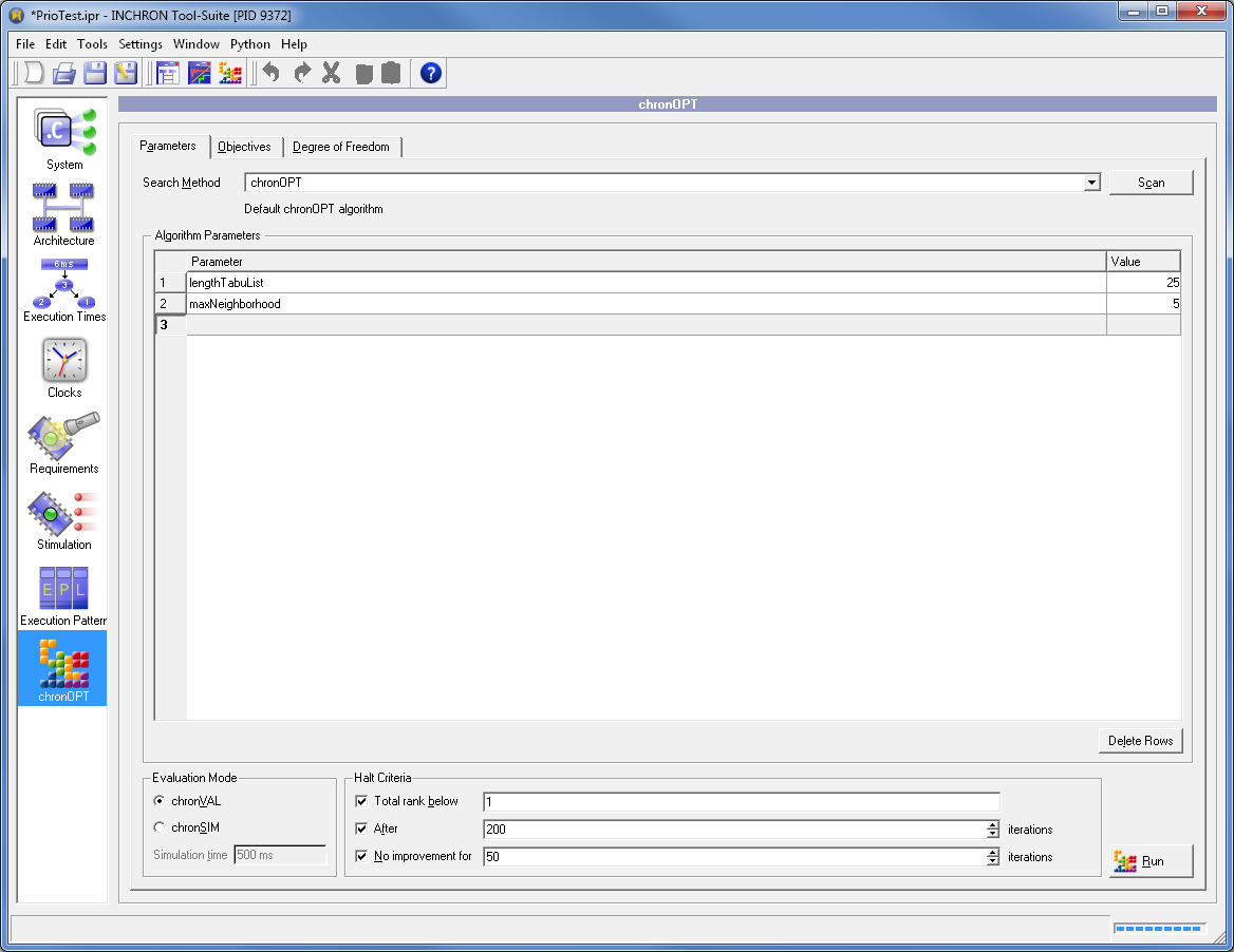
Figure 9.3: chronOPT Parameters tab of chronOPT example PrioTest.ipr #
In order to make chronOPT resolve this optimization problem by adjusting task priorities, the project is configured with an appropriate active Degree of Freedom and two Objectives.
Tip:
Since running chronOPT multiple times on the same project potentially yields different random solutions, a valid use case is to perform multiple runs of chronOPT on a initial system model in order to explore alternative solutions for a given set of constraints (as defined by the objectives).
E.g. with task priorities as degree in freedom alternative priority assignments each representing a viable solution (i.e meeting the requirements) may be explored.
Objectives for Optimizing Task Priorities#
The optimization goal is to minimize response times of the first four tasks. This is already expressed by four response time requirements for these tasks. Hence one could assume, that chronOPT just employs evaluations of these real-time requirements as the multi-objective cost function of the optimization. In fact, objectives of chronOPT optimization are configured separately from real-time requirements for purpose of more flexibility regarding additional objective types. I.e. chronOPT not only allows the use of real-time requirements as objectives but also several other types of objectives specific to certain optimization use cases.
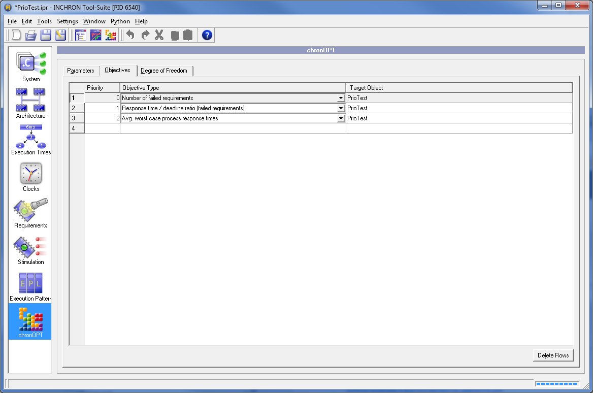
Figure 9.4: Objectives of chronOPT example PrioTest.ipr #
Degree of Freedom for Optimizing Task Priorities#
The object variables are the free parameters of the system model as defined on tab Degree of Freedom. For the specific use case of varying task priorities in a specified scope (e.g. of a certain scheduler or CPU) there is a dedicated type of Degree of Freedom which is applied on that example project.
An additional Degree of Freedom targeted at assigning tasks to processor cores is also configured but initially inactive. Hence all tasks are bound to a single core as defined by the Process Affinities.
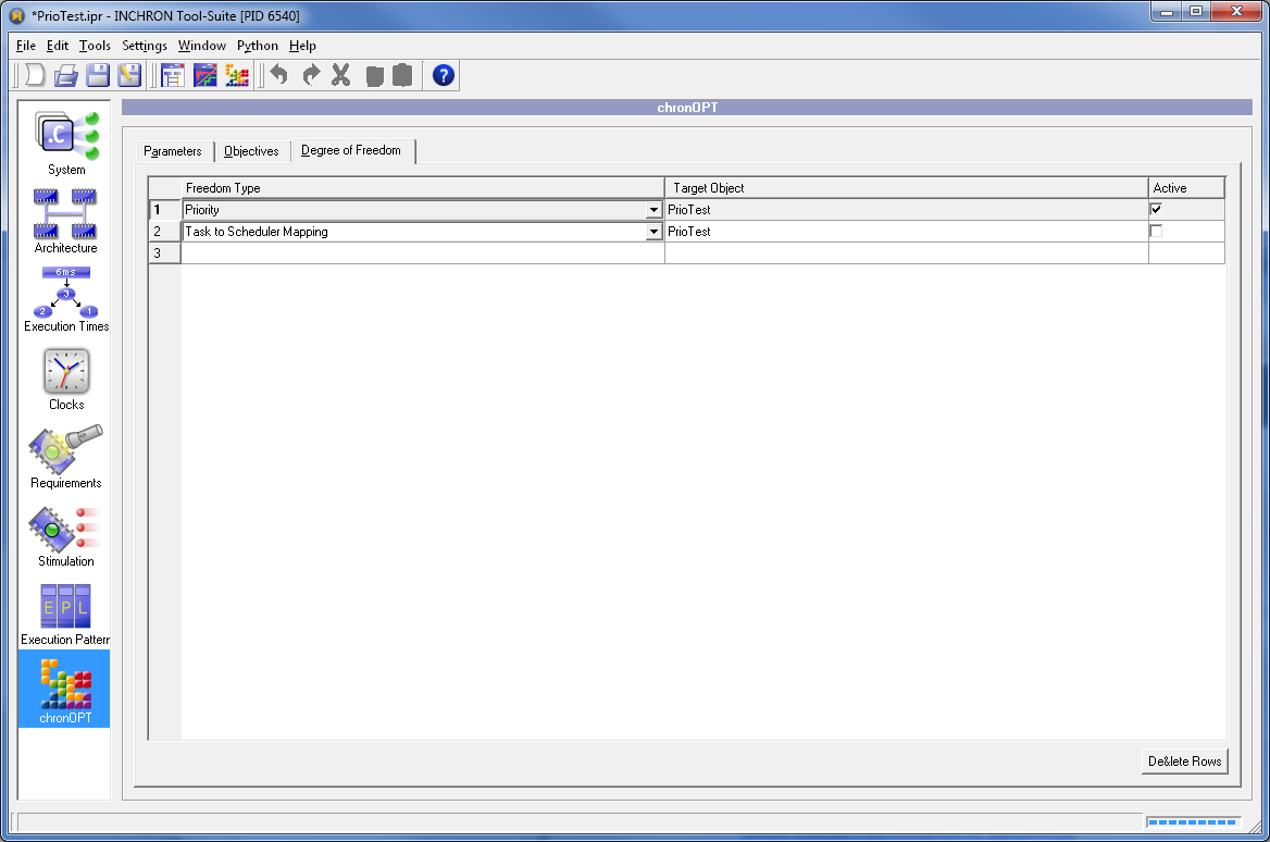
Figure 9.5: Degree of Freedom of chronOPT example PrioTest.ipr #
9.1.1 Running the Task Priorities Optimization #
By running the optimization priorities will be adjusted randomly and iteratively until meeting all requirements which have been specified as objectives The optimization will also stop if one of the Halt Criteria on the Parameters tab is met.
Click the button to start the optimization and launch the Optimizer Window as shown below.
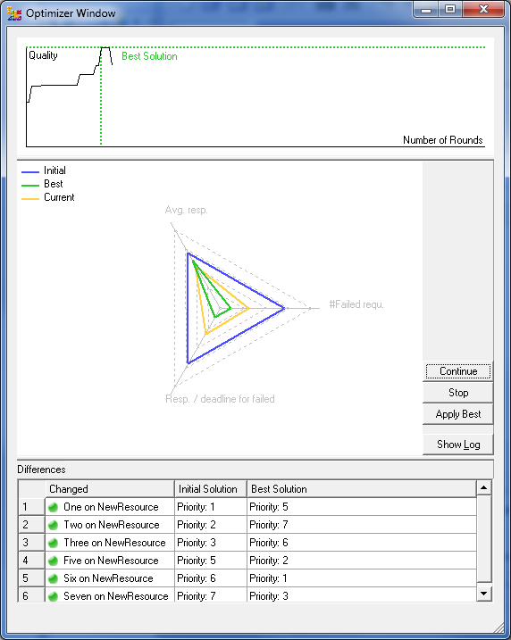
Figure 9.6: Optimizer Window for chronOPT example PrioTest.ipr #
The Optimizer Window will show two diagrams, the first indicating optimization progress and the second showing evaluations of all objectives as a radar chart and also a table of applied system model changes.
Optimization Progress Graph#
The first diagram of the Optimizer Window shown in Figure 9.6, “Optimizer Window for chronOPT example PrioTest.ipr” is a graph of overall quality over time, i.e. a metric which is a scalarization of objective evaluations of the best solution found in each iteration (with higher values indicating less overall violation of objectives). The overall best solution is indicated with green dashed lines. The Best Solution indicator relates to the Best graph in the spider chart.
Important:
Due to the ranking mechanism of the chronOPT algorithm, the best solution is not always the one with the highest quality value.
Objectives Evaluation Chart#
The second diagram of the Optimizer Window shows a radar chart with one dimension for each objective. The polygon shaped graphs in this diagram represent objective evaluations of intermediate system model variants during optimization.
The three graphs represent evaluations of individual objectives for the three particular solutions at optimization start, best solution of the most recently finished iteration and overall best solution during optimization. Since objective evaluations are in terms of errors (in contrast to quality), big polygons represent solutions of low quality. Hence the polygon representing objective evaluations at optimization start is usually the biggest and the polygon representing the most recent iteration will be shrinking as the optimization converges to better solutions over time.
Table of System Model Changes#
The table in the lower part of the Optimizer Window shows the differences between the initial system model and the current best solution. Each row of the table represents one changed attribute of the system model with the left column designating the object which has changed and the two adjacent columns showing the old and new value of the attribute.
9.1.2 Optimizing Task to Core Assignment #
The goal of minimizing task response times may also be achieved by appropriately assigning tasks to processor cores. In the example project, the optimization can be instructed to do just this:
First, if the example project has been changed by a prior optimization run, load
doc/examples/chronOPT/PrioTest.ipragain via → .Select the Degree of Freedom tab
On this tab, select the second table row, click the Freedom type column and select Task to Core Mapping from the drop-down list, as shown below.
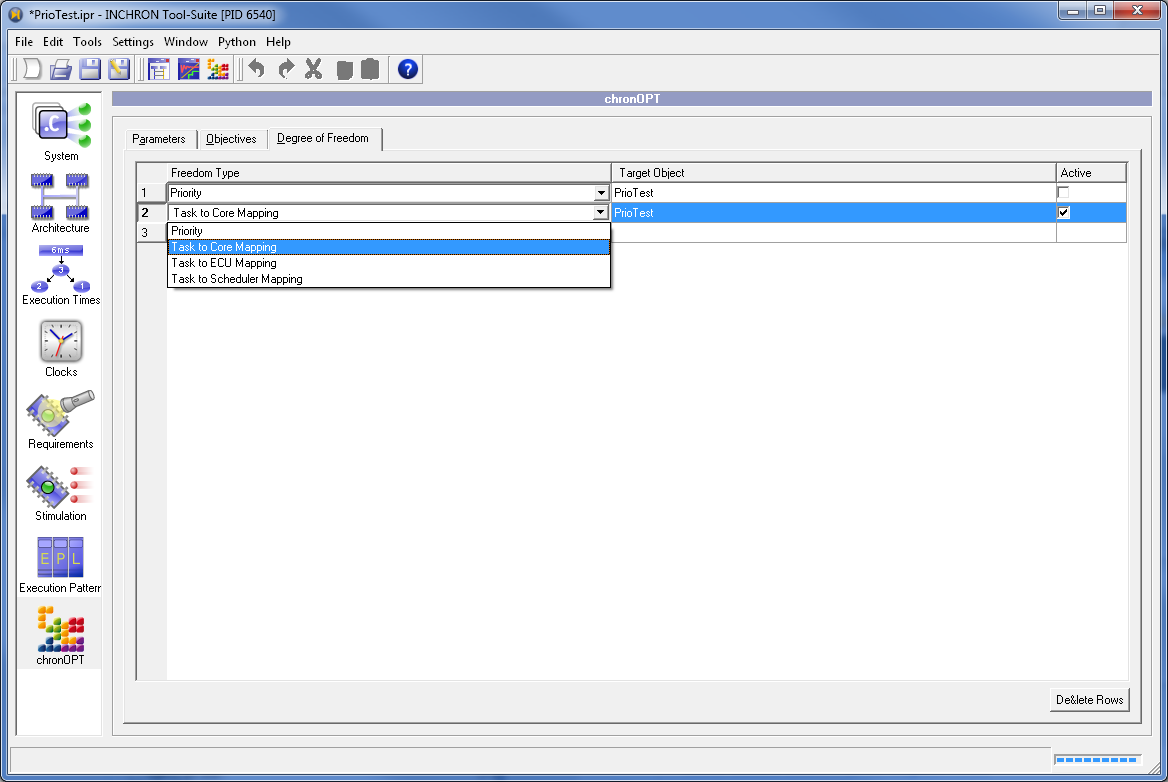
Figure 9.7: Degree of Freedom for Task to Core Assignment #
Then check the active option on the Task to Core Mapping degree of freedom and
un-check the active option on the Priority degree of freedom.
Finally, select the Parameters tab and click Run to start.
When running the optimization, solutions satisfying the given objectives will be found much quicker than by priority changes because distributing tasks on an additional core is obviously a more straightforward optimization problem.
Of course, it is also possible to activate both degree of freedom at the same time. As result, when running this on the initial project (mind to reload if necessary) a valid solution will be found even faster. The Optimizer Window screenshot below shows that a good solution is found within a few iterations and the table of applied modifications shows changes for both task priorities and task to core assignments.
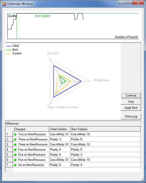
Figure 9.8: Optimization Progress for Task to Core Assignment #
9.2 Objectives #
The optimization goals are described with one or more Objectives. All defined objectives are commonly evaluated by either chronVAL analysis or chronSIM simulation. In chronOPT the concept of objectives is related to real-time requirements. But instead of just defining minimization of the projects real-time requirements this concept is more flexible. There are a number of predefined objective types, with one type in fact allowing to specify any Real-Time Requirement as an objective. I.e. the optimization will strive to minimize violations of this requirement.
Each objective type is targeting one or more system model element of specific types, like e.g. a CPU resource.
- Real-time Requirement
Valid objective target is a real-time requirement. The objective will evaluate as one in case of requirement violation and as zero else.
- Number of failed requirements
Valid scope (objective target) is either the project or a requirement group. This objective evaluates to the number of failed requirements in the scope (independently of how often they fail and the actual deviation from requirement limits) [19].
- Response time / deadline ratio
Valid scope (objective target) is either the project, a requirement group containing response time requirements [20] or a specific response time requirement. This objective evaluates the average response time to deadline ratio of the response time requirement(s) (with the deadline given by the requirement time limit).
- Response time / deadline ratio (failed requirements)
This is the same as above with the difference, that only ratios of requirement violations are evaluated.
- Average process response times
This objective evaluates as the mean response time of all processes in the selected target scope. In case of chronSIM as evaluation method response times of multiple simulated executions will also be averaged.
- Average message response times
This objective evaluates as the mean response time of all messages in the selected target scope. In case of chronSIM as evaluation method response times of messages being sent multiple simulated will also be averaged.
- Average Load
Valid target objects are just the project, a CPU resource, a scheduler or a process. In case of a project the load of all its CPUs will be considered and in case of a scheduler all its processes accordingly.
9.2.1 Objective Prioritization #
An optimization even for simple system models usually requires the definition of multiple objectives in order to get all effects of model variation under control. The evaluation of optimization objectives will not be weighted after evaluation. Therefore, in order to prioritize certain objectives each objective will have an editable priority value. Objectives with the lowest priority value will have the highest precedence.
9.3 Degree Of Freedom #
The object variables to be used for a chronOPT optimization of as system model are part of the project's chronOPT configuration. Possible types of object variables are e.g. the modification of task priorities or scheduling parameters. The optimization will only apply the activated modifications in order to meet the requirements on the system model's real-time behavior.
These types and their parameters are defined independently of objectives on the Degree Of Freedom tab of the chronOPT configuration widget.
chronOPT provides several types of Degree Of Freedom, each describing two dimensions, the kind of variable to be modified and a scope or target regarding the system model to be optimized.
Multiple Degree Of Freedom may be defined as a list. Each type of Degree Of Freedom may be used more than once with different scope, facilitating flexible constraints on the scope, e.g. to apply for certain CPU resources and to exclude others.
- Priority
With this degree of freedom priority of tasks, ISRs or runnables will be selected as the object variables of the optimization. The scope may be limited to an individual task, etc. or to all tasks, etc. of a scheduler, CPU resource or the whole project. This type of modification is implemented as swapping priorities of two random tasks (i.e. not by just in- or decrementing the priority value of one task).
- Task to Core Mapping
This Degree of Freedom is for optimizing the mapping of tasks or ISRs to processor cores. [21] The scope may be individual or multiple tasks as with the Priority degree of freedom. Tasks will always be moved between cores of the same CPU only, even if the Project is specified as the scope.
- Task to Scheduler Mapping
This Degree of Freedom is for optimizing the mapping of tasks or ISRs to schedulers. Only moves between schedulers of same type will be considered. Processes will only be moved between schedulers of the same CPU resource (aka ECU).
- Task to ECU Mapping
This Degree of Freedom is for optimizing the mapping of tasks or ISRs between schedulers across CPU resources. Only moves between schedulers of same type will be considered.
The list of Degree of Freedom type will be extended in future releases.
9.4 Optimization Algorithm #
The search heuristic is implemented as a
tabu search (https://en.wikipedia.org/wiki/Tabu_search).
The tabu search aims to improve a current best solution iteratively.
For this purpose, system model variants (candidates) are generated
by randomly changing the current best solution
until either a an improved solution has been found
or up to maxNeighborhood
candidates have been evaluated.
This means the parameter maxNeighborhood
limits the number of evaluated candidates per iteration
which is of great influence on search depth and search time.
Hence for iterations where no improved candidate is found, the result of that iteration will be a deterioration. Any intermediate overall best solution will remain available as the final result of the optimization though.
Local system model variants are generated by applying random moves according to the defined set of Degree of Freedom.
9.4.1 Tabu List #
The tabu list is a queue data structure
storing certain moves from most recent iterations.
Whenever the result of an iteration of the optimization
does not represent an improvement over the last iteration,
the underlying move leading to that solution
will be pushed to the tabu list
(which is initially empty but has the maximum length lengthTabuList).
All inverse moves of the moves in the tabu list are excluded
as possible moves for upcoming iterations until they expire
(i.e. are popped off the tabu list as the result of pushing new moves).
9.4.2 Generation of Candidates #
In each iteration, the optimization will generate system model variants from the current solution, i.e. the current state of the project (system model) under consideration. For that purpose, in each iteration a list of possible moves will be generated based on the specified list of Degree of Freedom, defining a local neighborhood of possible candidate solutions.
Possible moves are internally represented as Move
i.e. as an incremental change,
like Exchange priorities of Task A and Task B.
The union of all these neighborhoods serves as a pool of new possible candidates for an iteration of the optimization. Moves are randomly selected from the combined neighborhood, considering individual neighborhoods with equal probability, i.e. independently of different sizes of individual neighborhoods.
Effect of the Tabu List#
Using a tabu list is a means to improve search space exploration
i.e. it prevents getting stuck in recurringly iterating the neighborhood of a local minimum
(for the case of an error minimization problem).
If e.g. a move like Map Task A on core 0 to core 3
has been pushed to the tabu list then any inverse move
i.e. Map Task A from core 3 to core 0
will be not be considered until banning of this move expires.
9.4.3 Ranking of Evaluated Candidates #
The ranking of up to maxNeighborhood system model variants
in each iteration is based on evaluations of optimization objectives.
Hence in case of multiple objectives, weighting or prioritization
of the vector of objective evaluations has to be applied.
For that purpose, the default implementation of the chronOPT search heuristics uses an objective precedence for that. This means, evaluations of individual objectives for two candidates are compared in the order of specified objective priority. As soon as the evaluations for an objective are different the ranking (decision about improved solution) will be based on evaluations of this objective and subsequent objectives will not be considered for these two candidates.
9.5 Search Customization #
Many aspects of the chronOPT behavior regarding optimization objectives and object variables (degree of freedom) are configured in the Tool-Suite UI. Since chronOPT is designed as an optimization platform with actual algorithms provided as python scripts even greater flexibility can be achieved by customizing the underlying python source code.
This means that the calculation of neighborhoods for certain Degree of Freedom and evaluation of objectives
may be customized.
Even custom search heuristics are possible by deriving from either the default implementation
or the generic Optimizer base class.
9.5.1 chronOPT Batch Processing #
Batch processing of multiple optimization runs may be performed using the
Batch.exe command line tool.
An optimization run without UI frontend is performed with a command line like
$ Batch [-S|--seed SEED] -c -p <path-to-suite-installation>/chronOPT/chronOPT.py <project-file>.
Identical values for the seed option may be used
to get reproducible (identical) optimization runs
on optimizations of the same project (as long as the optimization algorithm also remains unchanged).
Option -c is applied to prevent simulation of the
project after optimization (the specified optimization triggers
chronSIM simulaton or chronVAL validation of candidate projects as
specified in the optimization settings of the given project.
9.5.2 Parallelized chronOPT Runs #
Due to the nondeterministic nature of optimization algorithms
the outcome of a chronOPT optimization will depend of the applied random seed.
Often it will be necessary to do multiple optimization runs in order to find a suitable solution
or to explore different suboptimal solutions.
For this purpose a python wrapper script is provided
for the Batch optimization
for running multiple optimizations of the same project in parallel.
See Section B.3, “chronOptParallel Script” for usage details.
9.5.3 chronOPT Scripts #
The default python chronOPT script is provided as
chronOPT/chronOPT.py in the Tool-Suite installation directory.
This chronOPT script is just a small wrapper script being executed
from when invoking an optimization the Tool-Suite UI
(or with the Batch.exe command line tool).
It will then instantiate and run an instance
of an Optimizer class
(by default a TabuSearch)
from the chronOPT library.
Multiple such chronOPT scripts are supported and for that purpose
a chronOPT python script has a comment section with special formal key-value pairs,
the most important being # chronOPT: yes.
Every valid chronOPT script in this directory will be listed
in the Search Method drop-down list
on the Parameters tab
of the Tool-Suite's chronOPT configuration UI module.
9.5.4 chronOPT Library #
The python implementation of chronOPT is provided in python files in the
chronOPT/lib/ directory of the Tool-Suite installation.
- Class
Optimizer Base class for chronOPT optimization algorithms. This basically provides the central abstract method
optimizationRound()This method is to be implemented in derived classes and will be called iteratively until a halt condition is met.- Class
TabuSearch Derives class
Optimizerand implements optimizationRound() as a tabu search.- Class
Move Base class for describing an incremental change on a system model. For any system model a degree of freedom defines a local neighborhood which is represented as a set of
Move.- Class
Neighborhood Base class for generating
Movelists which are specific to a corresponding type of Degree of Freedom. Derived classes arePrioNeighborhoodfor the Priority degree of freedom,CoreNeighborhoodfor the Task to Core Mapping degree of freedom,ChangeMappingToSchedulerNeighborhoodandChangeMappingOfRunnablesNeighborhood.- Class
CombinedNeighborhood Class
Neighborhoodderived class which provides random choice ofMoves for multiple Degree of Freedom (i.e. their corresponding neighborhoods). ACombinedNeighborhoodis generated in each chronOPT iteration for purpose of randomly selecting candidates (system model variants) for objectives evaluation.
For API and implementation details see the class documentation of provided python scripts of the chronOPT library.
[19] In fact, the same evaluation behavior can be obtained with a real-time requirement by specifying the same requirement group (usually "All Requirements") as its target.
[20] In case of evaluation by chronSIM more generally any timing requirement will be considered for objective evaluation.
[21] This requires a CPU with a multicore target model.
10 Interactive Design of Dynamic Architectures #
Interactive design of the dynamic architecture allows to create the model from a behavioral point of view instead of the structural view as described in Chapter 6, System Modeling. The interactive design features of the simulator are aimed at timing architects to e.g. support the planning of execution schedules. Additionally, by changing task or runnable allocations the load can be balanced between processor cores and processors or distributed over time and easily visualized.
For that purpose the Simulator Window provides a set of operations to modify the system directly from within simulation diagrams. The effect of such changes can immediately be reviewed by in the Simulator Window by updating the simulation.
10.1 Methodology #
The principle behind interactive design is to use the simulator to unreel the behavior of the system immediately after every change, to update the visualization, and to offer the most important changes from within the diagrams.
There are two possibilities for changes:
-
Within a diagram the user can open the context menu and select Change. Any change from there will update the simulation while keeping the stimulation scenario and the Control Window settings.
-
All changes from Chapter 6, System Modeling do not immediately update the diagrams. This is deferred until the user clicks on Generate Simulation or Run Simulation.
To start the interactive mode a minimal system with at least one process is required (otherwise there would be no diagram and thus no context menu). Follow these steps to start the interactive mode:
-
Start with an empty project by clicking on New Project.
-
Add a resource to the project.
-
Add a process to the default scheduler.
-
Click on Generate Simulation.
A message box appears claiming that the process has no execution time specified.
-
Click on Continue generation.
The Simulator Window opens.
-
Click on Show/Hide State Diagram to open the State Diagram.
The State Diagram opens. It show the defined process with no activity.
Now you can start to edit the model interactively by opening the context menu of the State Diagram an selecting Change.
10.2 Changing the Model #
The following changes are available from the context menu of a diagram:
Edit
Set Core Affinity
Map to Other Resource
Add Resource
Add Process
Remove Process
Add Incoming Dependency
Add Outgoing Dependency
Add Activation Here
The Simulator Window has no individual buttons for undo and redo. Use the buttons in the Project Mode Window instead.
Not every change is possible from within every diagram. Changes specific to a process can only be made in the State Diagram. Other diagrams offer only to add processes and resources.
10.2.1 Edit #
The Edit Process Dialog shows the basic properties of the process like execution time, simulation replacement, priority, and preemption. Any change made there will update the simulation with the new properties.
10.2.2 Set Core Affinity #
This menu entry is only available on multicore resources. It shows the Edit Core Affinity Dialog for the selected process. Again every change made here will be reflected in an update simulation.
10.2.3 Map to Other Resource #
This moves the process to another resource. When selected the Map to Resource Dialog will be shown. There you have to select a new scheduler where the process will be added.
10.2.4 Add Resource #
This adds a new resource to the model. You have to enter a name and to select a processor model. As the resource initially has no process no new diagram will be shown in the State Diagram after the update.
10.2.5 Add Process #
A new process will be added. The same dialog as with Edit will be shown but you have to enter a name and to select a resource, too.
10.2.6 Remove Process #
The selected process will be removed from the model without further question. If you need to undo this use the Undo Button in the Project Mode Window.
10.2.7 Add Incoming Dependency #
This adds an incoming dependency to the selected process. In the dialog you have to select the source of the dependency, and if it activates the receiver (otherwise it is a data dependency). Additional properties of the dependency can be edited in the Project Mode Window.
10.2.8 Add Outgoing Dependency #
This adds an outgoing dependency to the selected process. All outgoing dependencies are activated when the process has executed. As for an incoming dependency you have to select a receiver and if the receiver is activated.
10.2.9 Add Activation Here #
A newly created process is not activated except for the Activate At Boot option. With the Add Process Activation Dialog you can add more activations. The point of time is prefilled with the point where you clicked in the diagram. Optionally a period repetition can be specified. Further options for activations are available in Section 6.7.2.3, “Selecting the Target”.
10.3 Relation to Simulator and Validator #
10.3.1 Types of Models #
Models created by the interactive mode offer a lot of functionality without the need to add source code behavior for processes and runnables. Existing models with source code can also be modified (which implies that the execution time of functions is given by the exectuted instructions (if not overridden by a simulation replacement)).
10.3.2 Integration with the Simulator #
The interactive mode uses the simulator to immediately update the diagrams. Naturally all diagram types are available in this mode, including the Load Diagram, the Histogram, and the HTML Report.
10.3.3 Integration with the Validator #
When you create models interactively they do not contain source code by default. Therefor these models can also be analyzed with the Validator. See Section 8.1, “The Validation Concept” for details.
The validator also offers a interactive change of the analyzed model. With the Sensitivity Analysis in the Event Spectrum Viewer the user can change the execution time and activation frequency of processes efficiently.
11 Integration with IBM Rational Software #
11.1 Integration with IBM Rational Rhapsody #
11.2 Integration with IBM Rational DOORS #
One of the key elements of successful development projects is the acquisition and tracing of requirements. While INCHRON Tool-Suite offers the definition and evaluation of real-time requirements as a core feature it relies for these process activities on an external requirement management tool like IBM Rational DOORS.
11.2.1 Installation and Configuration #
The connection to the IBM Rational DOORS server uses OSLC (Open Services for Lifecycle Collaboration). It needs to be configured before use (see Section 2.4.2, “Configuration”).
11.2.2 Importing Requirements from DOORS #
The Tool-Suite also supports the import of requirements from DOORS®. Each requirement imported from DOORS is treated in the Tool-Suite as a text-based, informal container (requirement group) without possibility for evaluation on its own. The native real-time requirements of the Tool-Suite are added to such a container to facilitate the evaluation of the DOORS requirement. The combined result of these sub-requirements is used as status of the imported requirement and can be sent back to DOORS.
11.2.2.1 Prerequisites #
The connection between the Tool-Suite and DOORS uses OSLC. This requires the installation of DOORS Web Access and the configuration of the Root Services URL.
See Section 2.4.2, “Configuration” for details on the required DOORS version and the configuration.
11.2.2.2 Principle of Usage #
The workflow between the Tool-Suite and DOORS uses the delegated user interface of the DOORS Web Access, e.g. for the user authentification. If such interaction is required, the Tool-Suite automatically starts an external web browser. When the interaction in the web browser ends, the workflow returns to the Tool-Suite.
11.2.2.3 Import and Update of Requirements #
To import or update requirements from DOORS follow these steps:
-
In the MainWindow of the Tool-Suite select → → .
A browser opens. Depending on previous actions it may show the login screen of the Doors Web Access.
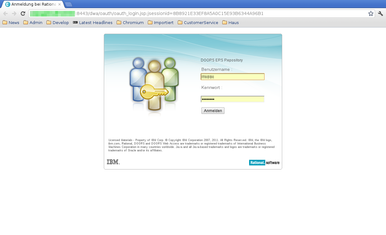
-
Enter your credentials.
Once your are logged in, a selection screen shows.
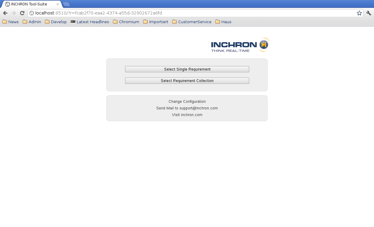
-
At this point you can either select a single requirement for import or a collection of requirements.
In both cases the delegated user interface of DOORS allows you to select a specific item.
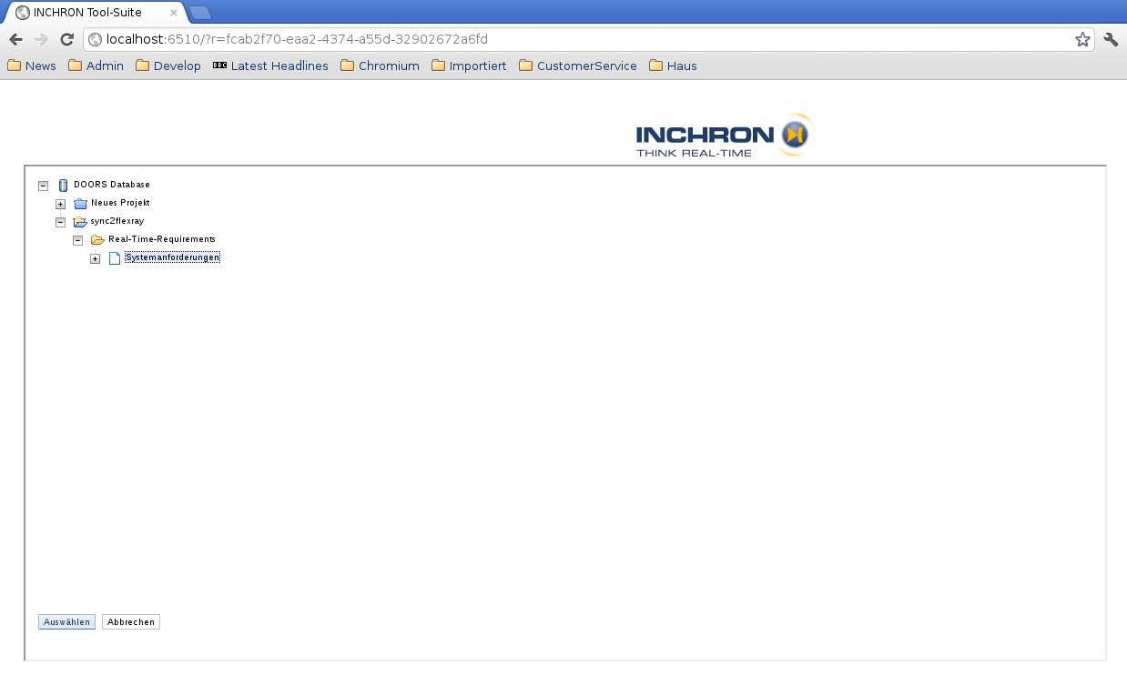
-
Select your intended item and click on Select.
The next page appears.
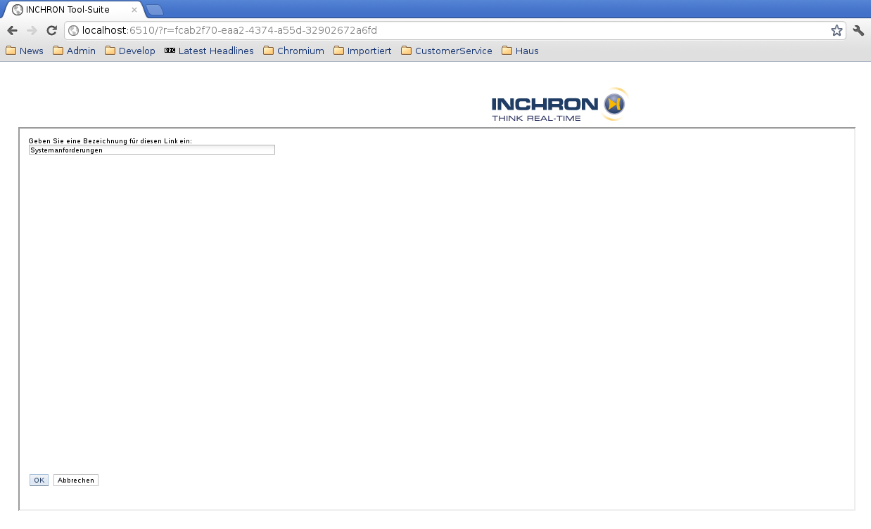
-
You are requested to enter a name for the imported requirements. Enter a name and click on Ok.
The import has been completed. You can now close the browser and return to the Tool-Suite.
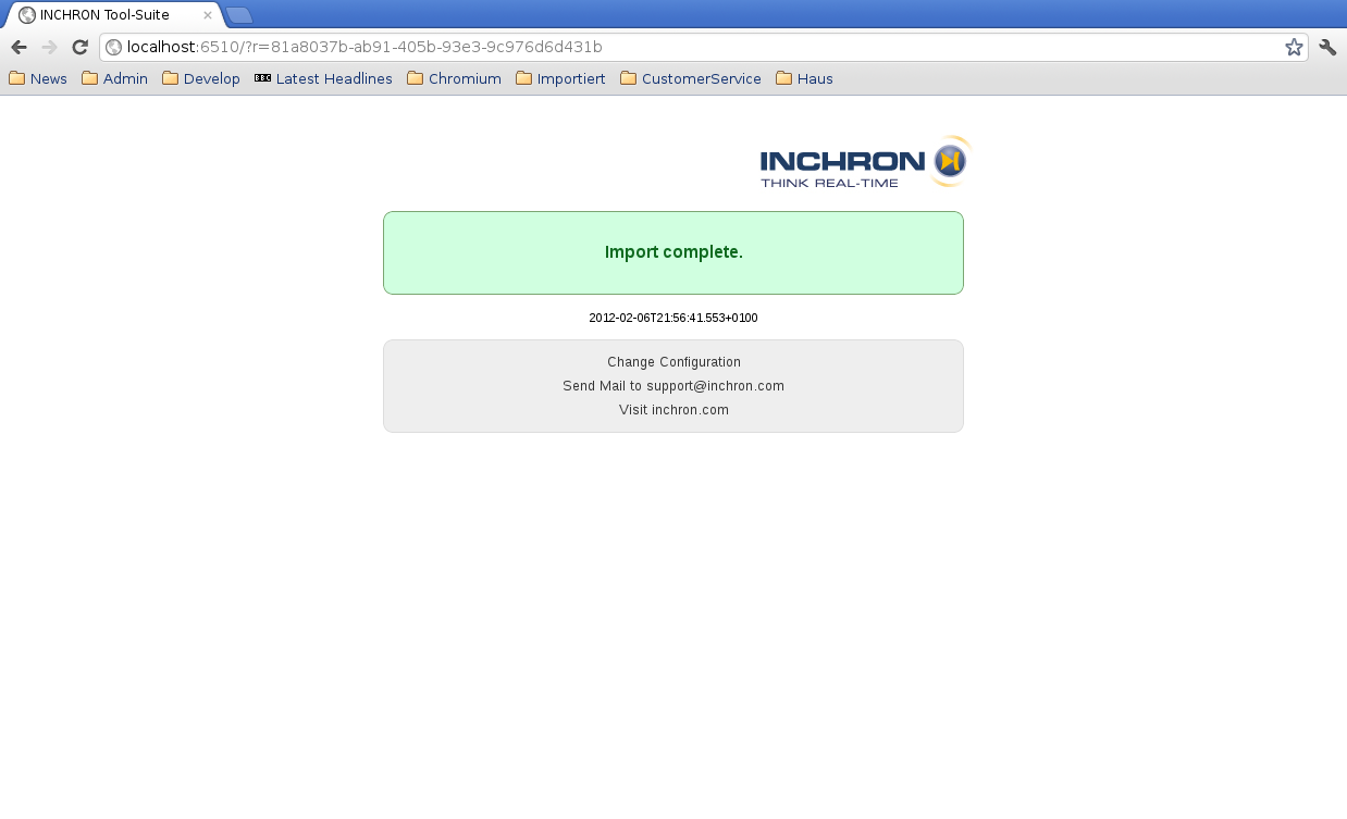
-
The requirements are now imported into the Tool-Suite.
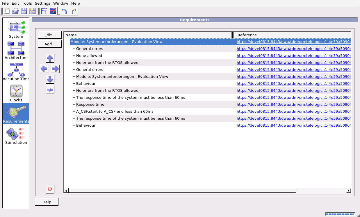
Each DOORS requirement is imported as an empty Group of Requirements. It cannot be modified. Realtime-requirements can be added as sub-elements for the purpose of evaluation.
11.2.2.4 Export of Requirements #
See Section 11.2.4, “Export and Update of Requirements to DOORS” on how to export the results of a simulation or validation to DOORS.
11.2.3 Refinement of Requirements #
Requirements in a requirements management tool like DOORS are usually plain text and very informal. Contrary to this a real-time requirement needs to be very specific and technical to be evaluated automatically with tools like chronSIM and chronVAL. To close this gap the Tool-Suite supports the following mechanism:
-
Requirements imported from DOORS are treated as leader of a group of real-time requirements. The show the same title as in DOORS and reference the DOORS requirement with its unique id.
-
The user groups specific real-time requirements below the DOORS requirement. Any number of requirements can be used to describe the DOORS requirement technically.
-
During simulation or validation all real-time requirements are evaluated and get a status of failed or passed. The result of the initial DOORS requirement is the logical merging of the stati of its children.
-
The results of the DOORS requirements can be written back to the DOORS database. They can be shown if defined as view in DOORS.
11.2.4 Export and Update of Requirements to DOORS #
11.2.4.1 Prerequisites #
The connection between the Tool-Suite and DOORS uses OSLC. This requires the installation of DOORS Web Access and the configuration of the Root Services URL.
See Section 2.4.2, “Configuration” for details on the required DOORS version and the configuration.
11.2.4.2 Obtaining Simulation Results #
After importing informal requirements from a DOORS database (see Section 11.2.2, “Importing Requirements from DOORS” for this) they need to be refined by technical requirements. Select the DOORS requirement and add a matching requirement from the list. Once this is done the simulation can be run which gives results similar to the following picture.
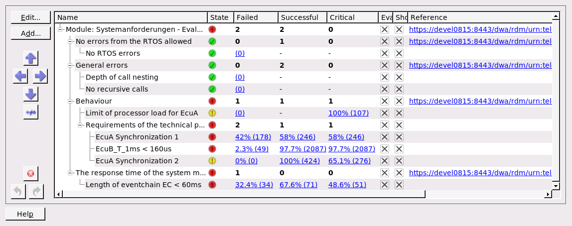
Figure 11.1: Requirement evaluations after import from DOORS and refinement #
During simulation and validation the requirements are evaluated automatically. The results of these evaluations can be exported to the DOORS database.
11.2.4.3 Starting the Export to DOORS #
The export is started from the Simulator Window with →
For each requirement group which was created by the import from a DOORS database and which has a reference to the corresponding database entry the status of their children are concatenated into a text message. This text is added to the database entry in the attribute which is specified in the DOORS configuration (see Section 2.4.2, “Configuration”). It contains an abbreviation of the technical requirement, its current status, information about the project, and the timestamp of the simulation.
11.2.4.4 Conflict resolution #
Before committing the export to DOORS it is checked if the requirements have been modified outside from the INCHRON Tool-Suite. If there are conflicting changes the user has to resolve the conflicts manually. Conflicts are shown in a way like this:
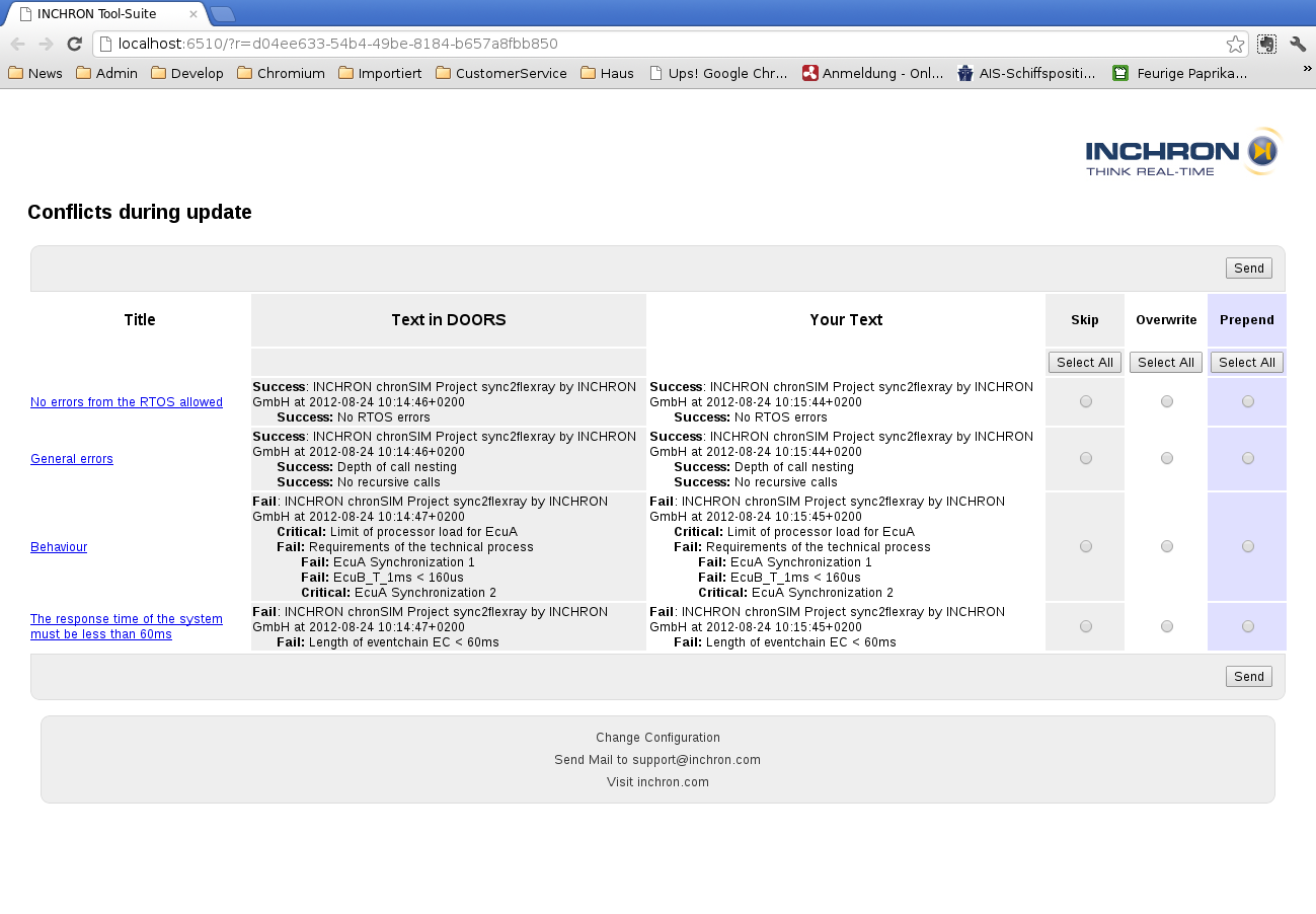
Figure 11.2: Conflicting changes detected during export to DOORS #
As a conflict resolution strategy the user can select between append of new results, prepend of new results, and overwriting the previous content. This can be selected either for all requirements or for each individually. When done press to continue. When everything went well a positive message is shown. This page can be closed.
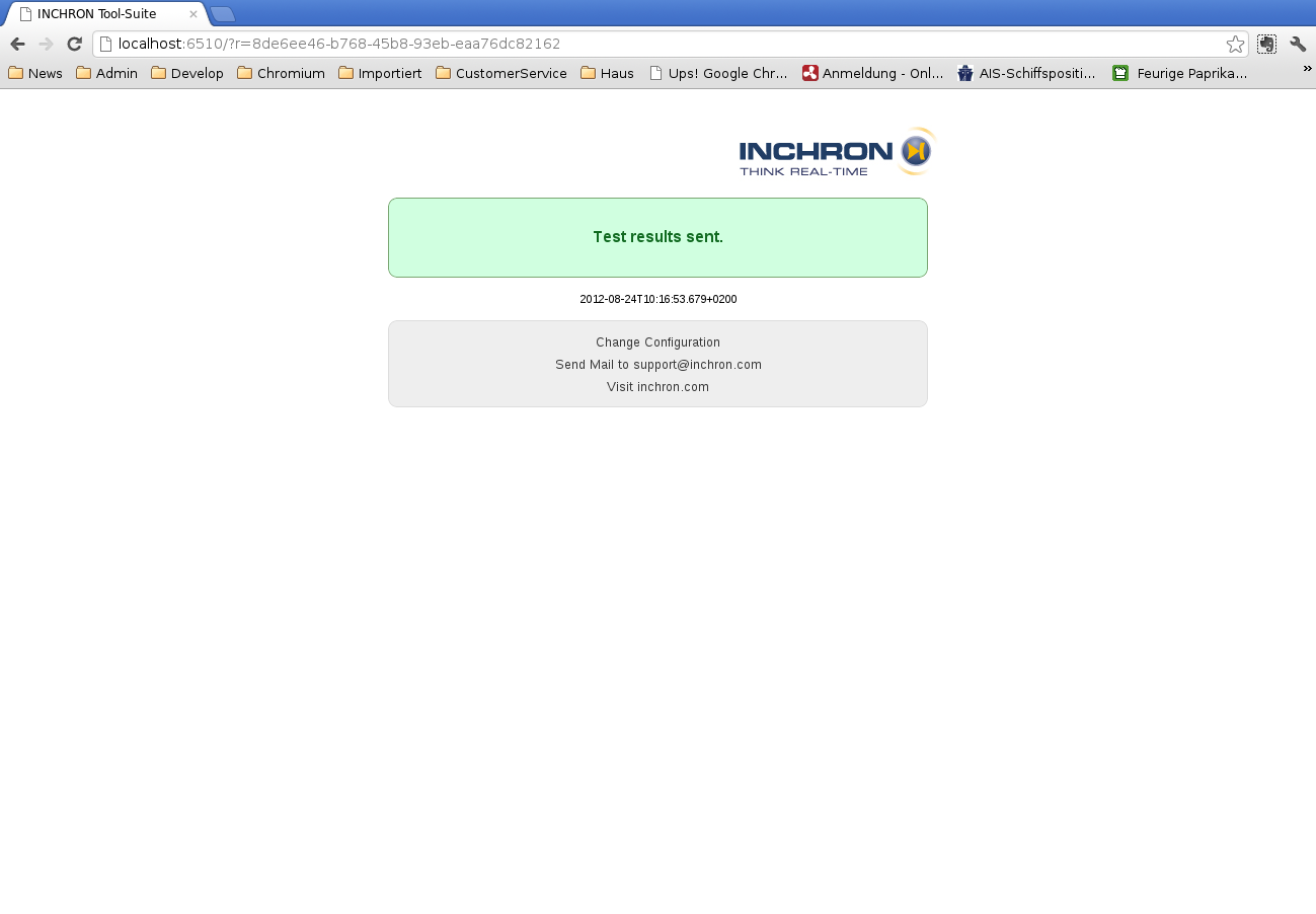
Figure 11.3: Status page shown after successful export to DOORS #
11.2.4.5 Requirement Evaluations in the DOORS Database #
An example of requirements and their simulation results is shown in the following screenshot from the DOORS Web Access. To the left are the usual columns showing the requirements and their numbering. In the right column titled Simulation Results the results obtained by the INCHRON Tool-Suite are shown. The name and visualization of this column has to be configured in the DOORS database. Contact your DOORS Database Adminstrator for doing this.
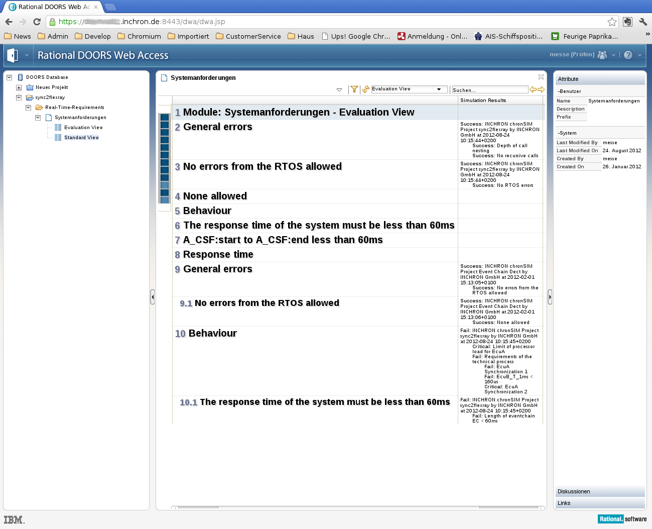
Figure 11.4: Viewing the requirements in the DOORS Web Access #
12 Subversion Integration #
The Tool-Suite features subversion client integration for certain use cases of version control (VC), i.e. for INCHRON projects, real-time requirements and simulation trace files as described in subsequent sections.
12.1 Setup Subversion #
12.1.1 Installation Requirements #
Not all requirements for version control are implemented in the Tool-Suite. For example, the subversion server and the password database are not integrated in the Tool-Suite. The Tool-Suite just invokes a subversion client installed on the host and subversion authentication services provided by the OS.
12.1.2 Setup of a Subversion Server #
Any subversion server can provide access to multiple SVN repositories.
Each repository has its own revision counter.
Different access permissions can be configured for each repository
and for individual directories in a repository
(albeit with higher configuration effort).
The Tool-Suite can access any subversion repository
for which the user enters the path.
This usually will be a HTTPS URL, but a
file:///path/to/localrepository
local file URL is also possible.
Important:
If you set up a subversion repository where trace archives shall be stored,
the server side setup requires a second subversion repository named
.archive on the same level.
This archive repository stores the large binary trace files
while the first user visible repository stores INCHRON trace archives
(with the extension .ita)
which contain an outline of the simulation trace and a reference
to the binary trace data
(.isf and
.idx) file)
located in the
.archive repository.
12.1.3 Setup of a Subversion Client #
The Tool-Suite relies on an external svn client executable to communicate with the subversion server. This provides flexibility regarding the subversion release to be used (which may differ in the format of the working copy layout). If you do not already have a svn executable installed on your workstation we recommend the installation of the TortoiseSVN plugin for the Windows explorer which is available from the Subversion website (http://tortoisesvn.net/index.de.html). It integrates nicely in the Windows Explorer and allows subversion operations on the file system outside of the Tool-Suite.
Important:
When installing TortoiseSVN please take care to also install the command line
tools (which usually will end up in
C:\Program Files\TortoiseSVN\bin folder).
Note:
By default Tool-Suite uses the svn.exe
which is found in the user’s %PATH%.
You may need to change this in the Tool Settings dialog
( → )
by selecting the svn.exe
in the bin folder of the TortoiseSVN installation
(usually C:\Program Files\TortoiseSVN\bin\svn.exe).
12.2 Repository Browsing and Operations #
Within the Tool-Suite navigating a subversion repository for either reading or writing is done via the the Repository Wizard. The Repository Wizard is commonly used for SVN transactions with the Tool-Suite to guide through the steps of Repository selection, optional authentication, browsing a repository directory, selecting a target file or directory and finally performing the desired repository operation.
First you need to provide a server side URL for the remote repository as shown below
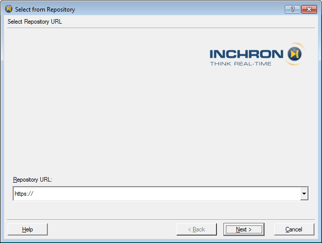
Figure 12.1: Repository Wizard #
After confirming with in case the repository is accessed for the first time the wizard will ask for user credentials:
Figure 12.2: Repository Authentication #
Enter your username and password and confirm with . The Tool-Suite will then pass the entered data to the external SVN client. If the login succeeds the operation proceeds. The username and password is stored by the external SVN client, it will not be stored by the Tool-Suite.
The next page of the wizard provides browsing of the repository directory tree on the server in order to select a target file object (e.g. an archived trace to open). As final step of the wizard, the desired VC operation (e.g. check out of a previously uploaded a project) is performed.
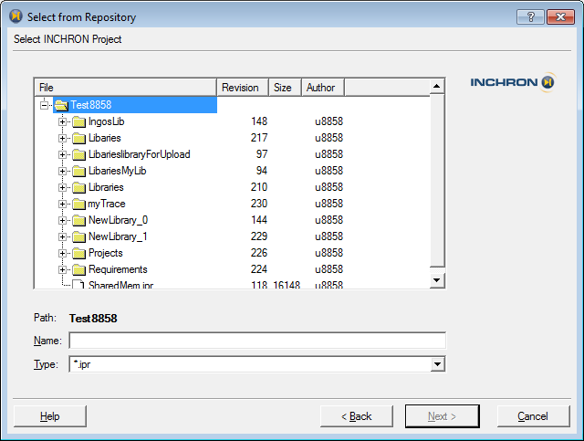
Figure 12.3: Repository Wizard #
You can clear the stored credentials as follows:
Browse the working copy with the Windows Explorer
In any directory open the context menu by clicking the right mouse button.
Select → as shown in the screenshot below.
In the Settings dialog select .
On the right hand side the button on Authentication data.
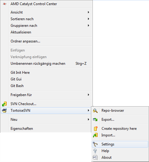
Figure 12.4: Access TortoiseSVN Settings #
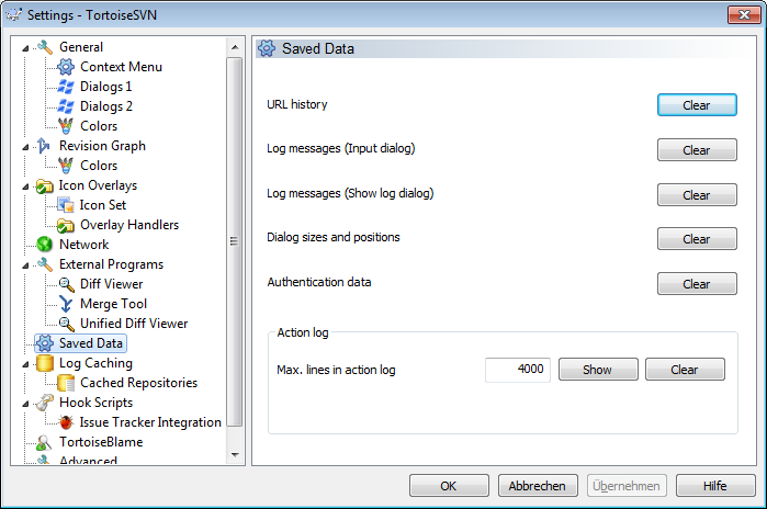
Figure 12.5: TortoiseSVN Settings #
12.3 Version Control for Projects #
All INCHRON projects can be put under version control (VC).
Tip: Location of Working Copies
Checked out working copies of INCHRON projects are stored in
C:\Users\%USER%\.inchron\Projects\.
12.3.1 Project Upload to a Repository #
An existing project can be put under version control by the following procedure:
Open the project.
Select → .
Enter the repository URL in the Repository Wizard and select a location for storing the project.
Optionally edit the commit message and press .
After initially uploading the project, modifications may be just committed via from the project item's context menu.
12.3.2 Open a Project from Repository #
To open a project from a repository follow these steps:
Select → .
Enter the repository URL in the Repository Wizard and select the project ipr.
Select a (relative) path for checkout of the project.
12.3.3 Work with Versioned Projects #
A project under version control shows an additional widget tab Version Control when the project item is selected in the system tree.
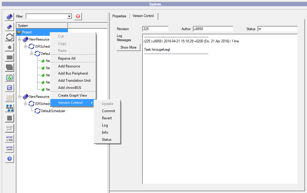
Figure 12.6: Version Control Information #
This widget shows the revision, author and log messages of the project under version control. The Status flags can show the following values:
status field is empty: the project is up-to-date.
'a' (added): the project was added to the local working copy. It is not yet part of the (remote) repository.
'm' (modified): the project was modified in the local working copy.
'u' (update): a newer version of the project exists in the repository.
Depending on the status different actions can be performed on the project. All possible actions are available from the version control context menu of the project (see screenshot above).
12.4 Version Control for Real-Time Requirements #
The Tool-Suite also supports import and export of real-time requirements from/to a subversion server.
For exported requirements the IRQ file format is used as described in
Section 6.6.13, “Import and Export of Requirements”.
Modification of existing IRQ uploads is currently not supported.
12.4.1 Upload to Repository #
For uploading of real-time requirements to a subversion repository use → which will launch a Repository Wizard.
12.4.2 Download from Repository #
Import of formerly uploaded real-time requirements is done with
→
In this case requirements from the IRQ file
may be optionally imported as a new requirement group.
When finishing the Repository Wizard a dialog will be shown which also allows to specify an additional textual import description. This description will shown in the tooltip of each requirement imported.
12.5 Version Control for Simulation Traces #
12.5.1 Upload a Trace to Repository #
Every simulation trace opened either in chronVIEW or in chronSIM can be archived to a subversion server.
Select the menu → .
The Repository Browser pops up and you are requested to select a subversion server.
Navigate to the location where you want to store the trace archive and enter the name with the extension
.ita. (INCHRON trace archive).[22]Enter a commit message and optionally additional information for the input fields Tracing Hardware, Tracing Date and Trace Comment.
The Tool-Suite then
creates and uploads an INCHRON trace archive (containing meta data and a reference to the binary trace data).
uploads the binary trace data to the separate remote
.archiverepository (which is not shown within the Tool-Suite UI).
12.5.2 Download a Trace from Repository #
Archived traces can be opened by:
selecting the menu → ,
and use the Repository Browser to select a trace archive (
.ita).
Tip:
This also works by dropping the URL of an
.ita
trace archive onto the Tool-Suite program icon.
The Tool-Suite then downloads the binary trace to the %TMP% folder
and opens it in chronVIEW. When the user closes this chronVIEW window the downloaded
trace file will be deleted automatically.
Additional information about the downloaded trace
(like trace comment or commit message) can be obtained by
→ .
A Technical Data #
The chronSIM real-time simulator comes along with the following technical characteristics concerning simulated hard- and software, 3rd part software and file formats:
A.1 Target Systems #
A.1.1 Target Platforms #
A target platform comprises a particular combination of CPU, compiler and operating system.
NEC V850, Green Hills Compiler, no RTOS
NEC V850, Green Hills Compiler, 3SOFT-OSEK
Motorola PowerPC 5200, GNU Compiler, no RTOS
Intel i386EX, GNU Compiler, no RTOS
Renesas M16C, IAR Compiler, no RTOS
A.1.2 Buses #
A.1.3 IO Peripherals #
A.2 Load Calculation #
The load diagram (Section 7.7.13, “Load Diagram”) and load requirements (Section 6.6.11, “Load Requirement”) both are based on the concept of continuous progression of the load of a CPU or bus resource over time.
The implementation of load calculation common for both is not based on the number of processes ready to be scheduled for execution as in Unix like operating systems but instead represents an equivalent of thermal power dissipation (not considering idle power though) produced by the activity of a processor in a given time interval.
While the resource power consumption is assumed as being either zero or 100%
at any given point of time the calculation of the continuous load value comprises the following steps
Equidistant load values are calculated by averaging actual load (being
0or100%, depending on resource activity) over a given granularity interval.Smoothed load values are calculated by applying a moving average filter of
nsteps (smoothing interval = n x granularity).Load between granularity steps is estimated by linear interpolation. [23]
A.3 INCHRON Tool-Suite File Formats #
- A.3.1 File Format of INCHRON Projects
- A.3.2 File Format of INCHRON Target Models
- A.3.3 File Format of Stimulation Scenarios
- A.3.4 File Format of Requirements
- A.3.5 File Format of View Profiles
- A.3.6 File Formats for Stimulation Data
- A.3.7 File Formats for Simulation Traces
- A.3.8 File Format for Reports
- A.3.9 File formats for Data Exchange
INCHRON Tool-Suite uses a number of file formats for internal use and for data exchange with other programs.
A.3.1 File Format of INCHRON Projects #
A.3.2 File Format of INCHRON Target Models #
Supported microprocessor target models are described in Appendix A, Technical Data, see also Section 6.2.6, “Microprocessors”.
A.3.3 File Format of Stimulation Scenarios #
A.3.4 File Format of Requirements #
*.IRQ: INCHRON real-time requirements as described in Section 6.6.13, “Import and Export of Requirements”
A.3.5 File Format of View Profiles #
A.3.6 File Formats for Stimulation Data #
*.CSV (see the section called “Read from CSV File”)
*.TXT
A.3.7 File Formats for Simulation Traces #
*.ISF: INCHRON simulation trace data
*.IDX: INCHRON simulation trace index data. In case an IDX file gets lost it may be recreated from the ISF with the traceconv tool.
*.ITA: INCHRON Trace Archive
A.3.8 File Format for Reports #
A.4 Third Party Software #
At runtime INCHRON Tool-Suite makes use of various 3rd party software packages. Proper operation of chronSIM will not be impaired if these software packages are not installed on your computer.
A.4.1 File Tools #
A.5 Compiler #
The following compilers are supported by default.
The integration of support for additional compilers introducing new C key words into chronSIM can only be provided by INCHRON.
B INCHRON Tool-Suite Command Line Tools #
Apart from the graphical user interface, the INCHRON Tool-Suite comes along with three additional tools intended for command line usage.
Batch.exe runs chronSIM simulation or chronVAL validation on a given INCHRON project. The ISF trace file resulting from a simulation may be analyzed with chronVIEW or converted to CSV using the traceconv tool. traceconv.exe converts this simulation trace to a CSV table.
The OILConverter.exe command line tool generates a INCHRON project file from an OIL specification file, which can be employed both for the graphical user interface of the Tool-Suite application as well as for the Batch.exe command line tool.
All command line tools are installed to the bin
subdirectory of your Tool-Suite installation path.
Batch.exe requires a valid chronSIM license to run;
traceconv.exe and
OILConverter.exe will work without a license.
All command-line tools are called from a command line with a set of parameters.
Each tool provides a --help parameter to print its own
help text containing a list of all possible parameters.
The usage of these command line tools are described in the following sections.
B.1 Suite.exe #
Suite.exe -- graphical user interface of INCHRON Tool-Suite
Starts the INCHRON Tool-Suite.
B.1.1 Usage #
Suite [-S|--seed SEED] [-N|-no-seed] [--screenshot]
      [-r|--run] [-u|--until ENDTIME] [-q|--quit]
      [--chronview|--chronsim|--chronval]
      [PROJECTFILE|TRACEFILE [n]]
Suite [-h|--help]
Suite [-V|--version]
B.1.1.1 Possible options are #
--chronview
Start the Tool-Suite in the chronVIEW mode. Will occupy only a chronVIEW license.
--chronsim, --chronval
Start the Tool-Suite in the Project mode. Will occupy a chronSIM and a chronVAL license if available.
-S, --seed=1234
Set seed value for pseudorandom numbers of stimuli generators This results in a deterministic sequence of stimuli for the projects active stimuli scenario.
-N, --no-seed
When a seed is set in the Settings -> Tool Settings Dialog it is stored in the registry. To request a simulation which ignores such a setting this option has to be used.
--screenshot
The size and the position of the MainWindow is stored between program starts. Use this option to enforce a standard size of 1152x864 when making screenshots.
-r, --run
Starts the simulation creation immediately after project loading has finished. The simulation then waits for user interaction.
-u, --until=TIME
Only usable together with --run. Runs the simulation until the
specified point of time. TIME has to be number and unit,
e.g. 500ms.
-q, --quit
Only usable together with --run. Quits the Tool-Suite
immediately after simulation creation or when the specified until time
has been reached.
PROJECTFILE|TRACEFILE [n]
When a project file with the extension .ipr is given it will be loaded. Trace files with the extension .isf are opened in chronVIEW. Specifying an integer number n loads the n-th recent project. Counting starts a zero.
-h|--help
Shows this help page.
-V|--version
Prints the release and build date and exits.
B.1.2 Examples #
$ Suite demo.ipr
Starts the INCHRON Tool-Suite and loads the project demo.ipr in the current directory.
$ Suite -r demo.ipr
Starts the INCHRON Tool-Suite, loads the projects, generates the simulation and opens the Simulator Window.
$ Suite 0
Starts the INCHRON Tool-Suite and loads the last project.
$ Suite 1 -r -u1s
Starts the INCHRON Tool-Suite, loads the second last project, generates a simulation and runs the simulation until a simulation time of 1s is reached.
$ Suite trace.isf
Starts the INCHRON Tool-Suite and loads the trace file trace.isf in chronVIEW mode.
B.2 Batch.exe #
Batch.exe -- batch processing of an INCHRON project
Performs chronSIM simulation, chronVAL validation or chronOPT optimization of a given IPR project file. No user interaction is intended during execution. The result of a simulation is an ISF trace file which may be analyzed with chronVIEW or converted to CSV with traceconv.
B.2.1 Usage #
Batch Simulation (chronSIM)#
Batch [-u|--until ENDTIME] [-o|--output NAME] [-I|--import-autosar]
		[-n|--num NUMOFRUNS]
		[-S|--seed SEED] [-N|--no-seed]
	    [-p|--python SCRIPT]
		[-s|--scenario SCENARIONAME]
		[-f|--format csv|btf]
		[-r|--report html|csv|ipr|extensive|buses | calltree|functionsall|functiontimes|requirements|requirementtimes|events]
		[-t|--template TEMPLATENAME]
		[-R|--requirements IRQFILE] PROJECTFILE | TRACEFILE
Batch Analysis (chronVAL)#
Batch -a|--analyze [-o|--output NAME]
		[-r|--report html|cvr] PROJECTFILE
Batch Optimization (chronOPT)#
Batch [-S|--seed SEED] -p OPTIMIZER-SCRIPT PROJECTFILE
(see Section 9.5.1, “chronOPT Batch Processing” for a description and.
Section B.3, “chronOptParallel Script” for parallelized execution).
Batch Processing of Project Files With a Python Script#
Batch -p|--python SCRIPT [-c ] [ --ipr RESULT ] [PROJECTFILE]
In case a PROJECTFILE (IPR) is given, specifying either -c or --ipr RESULT
will suppress subseqent simulation of the project.
Import of AUTOSAR ARXML#
Batch --import-autosar -c [--ipr IPR-NAME] ARXMLFILE
In case multiple arxml files shall be imported
ARXMLFILE may be specified as a directory which will be parsed recursively
for arxml input files.
Note:
With option -c subsequent simulation of the generated IPR is suppressed.
Import of a Custom CSV Trace File (chronVIEW)#
Batch -i|--import [-o|--output NAME] [-t|--template TEMPLATENAME]
	  [-r|--report html|csv|ipr|extensive|buses | calltree|functionsall|functiontimes|requirements|requirementtimes|events]
	  [-R|--requirements IRQFILE] CSVTRACE
Post-processing of Simulation Traces#
Batch -r|--report html|csv|ipr|extensive|buses | calltree|functionsall|functiontimes|requirements|requirementtimes|events
		[-R|--requirements IRQFILE] [-t|--template TEMPLATENAME]
		[-o|--output NAME] SIMTRACE
Checking Project Validity#
Batch -c|--check PROJECTFILE
Get Batch Help or Version#
Batch [-h|--help] [-V|--version]
Command Line Arguments and Options#
PROJECTFILEmeans an INCHRON project file (extension IPR).
TRACEFILEmeans an chronSIM simulation trace file (extension ISF).
ISLFILEmeans an INCHRON stimulation scenarios file (extension ISL) as described in Section 6.7.4, “Import and Export of Scenarios”
IRQFILEmeans an INCHRON requirements file (extension IRQ) as described in Section 6.6.1, “Concept of Module Requirements”
-a
Do chronVAL analysis (default is chronSIM simulation)
-p, --python SCRIPT
Execute given python script before simulation.
The script may create a project or modify the given PROJECTFILE.
Supply --ipr to specify a filename for the result IPR file.
This will also suppress subsequent simulation of the project (s.a. option -c).
The scripting option may also be used to invoke a chronOPT
optimization script.
-c, --check
Processing stops after parsing the project file. Neither the simulation nor a trace file is generated. This will yield exit code 0 in case of no errors.
-u, --until=TIME
Simulation stops when reaching specified point in time.
TIME has to be given as a value with time unit.
The value can be a float number without exponent; the unit has
to be one of ns, us, ms or s.
-o, --output=NAME
Name for output files (and report directory name).
NAME may be prepended with a path.
When omitting this option, the simulation will create a trace file
with the same basename as the input project in the current working directory.
For performance reasons avoid output to a remote share (NFS, SMB etc.)
The special name '-' is for textual output of the simulation trace to stdout.
The output to stdout cannot be combined with neither
--break nor --report.
See --format for available text formats.
See also --ipr for result IPR files.
-f, --format=csv|btf
Select alternative text output format for the simulation trace.
Currently supported formats are CSV and BTF with the former
being the default.
Direct output of the export format to STDOUT is possible
with e.g. -o -:csv instead of -f csv.
--numeric
BTF output: output trace entries with numeric IDs instead of symbolic names. Tables at the beginning of the output file allow the mapping of IDs to names.
--exclude STI,T,I,F,S,...
for BTF output only: do not show trace entries of given types (with STI: stimuli, T: task, I: interrupt, F: function and S: signal flow entries).
--include STI,T,I,F,S,...
for BTF output only: show trace entries of given types only.
-h, --help
Display this help and exit.
-i, --import CSVFILE
Import given custom CSV trace file and write it as an ISF file. The semantics of CSV columns has to be determined once prior to import by using the Tool-Suite's chronVIEW trace file import wizard as described in Section 7.8.3, “Trace File Import or Export”.
These settings are stored per import file ending, thus each distinct CSV
trace format requires a unique file ending (everything after the first dot)
for the input files. Alternatively, a custom CSV format settings file may be
provided by the user with option -P, --presetfile PRESETFILE.
--ipr
This option causes termination without simulation after script execution with
-p (which may be a chronOPT script).
This will yield the project passed from the script with the suite.set().
Without the -p scripting option, --ipr
may be used to just convert the input project to the current IPR version.
-n, --num=RUNS
After ending a single simulation another run is started until
a total of RUNS runs is reached.
The output files are named according to the pattern OUTFILE.%d.isf
where %d is the number of the single run.
-s, --scenario=SCENARIONAME
Runs the simulation with given scenario. This activates the specified stimulation scenario and overrides the default scenario from the project file.
--scenariofile=ISLFILE
Import stimulation scenarios from given ISL file.
If only one scenario is imported, it will be used in the simulation.
If the file contains multiple scenario definitions,
the default scenario or the scenario given by the --scenario
option is used instead.
-r, --report=html|csv|ipr|cvr|extensive|buses | calltree|functionsall|functiontimes|requirements|requirementtimes|events
Generates report of specified report type.
Multiple --report type specifiers may be combined.
Note:
Per default batch simulation reporting includes reporting for CPUs and their proecesses and functions, buses, events and requirements, overriding the report configuration stored within the given project file.
| chronSIM (simulation), chronVIEW (import) and direct ISF reporting support the following report format options: |
--report html generates a HTML report to a subdirectory
(default name 'report') |
--report csv summarizes report information in a CSV file. |
--report ipr will write report data to an IPR file. |
--report extensive will enable overriding IPR reporting
with a set of default reporting options (equivalent to --report buses,events,functionsall
and additionally event histograms, process and CPU load reporting). |
--report buses will include CAN and FlexRay message reporting |
--report calltree will write process and function execution times
to an IPR file. |
--report functionsallHTML and/or CSV report will include function
and call tree statistics anc call histograms. |
--report functiontimes HTML and/or CSV report will include detailed
execution time tables. |
--report requirementsHTML and/or CSV reports will include
evaluations of realtime requirements . |
--report requirementtimes HTML and/or CSV reports will include
detailed requirement evaluation time tables. |
--events HTML report will include
detailed statistics and histograms for EVENT1 and Transfer Counter values.
|
--report events HTML report will include detailed statistics
and histograms for EVENT1 and Transfer Counter values. |
--report none deactivates all previously set reporting options.
This is especially useful in combination with --break
which implicitly activates HTML requirement reporting. |
--with-report-unit=yes|no enables or disables the time unit
for the CSV report. |
--report-unit=s|ms|us|ns|ps|auto sets the time unit
for the CSV report (default is 'auto'. |
--report-precision=MIN,MAX sets the minimum
and maximum number of digits after the decimal mark for the CSV report. |
| chronVAL (analysis) reporting supports the following report format options: |
--report cvr generates a CVR (chronVAL result) file. |
--report html generates a HTML report. |
-t, --template=TEMPLATENAME
Specifies a template to be used for report generation (see Section 7.10.2, “Report Customization”. This overrides the report template selection from the project file.
-q, --quiet
Suppresses all console output.
-v, --verbose
Increases verbosity level. Default is level 1 which shows a progress bar in ASCII art.
-b, --break
Stops the simulation on requirement failure.
This also implicitly activates a HTML report with requirement reporting,
which can be suppressed by using a subsequent -r none.
Due to the simulation core being running simultaneously with the requirement
evaluation thread the actual simulation end will be some time after the
time of requirement failure.
-R, --requirements=IRQFILE
Adds specified requirements to be evaluated during report generation for simulations or imported CSV trace files. Project files will not be modified.
-S, --seed=1234
Set seed value for pseudo-random numbers of stimuli generators This results in a deterministic sequence of stimuli for the project's active stimuli scenario.
-N, --no-seed
When a seed is set in the Tool-Suite's
→
dialog this will be stored in the registry and used by
Batch.exe unless -N is given.
-V, --version
Display version number and exit.
Return codes #
0Everything went smooth. Project was successfully checked validator or simulation terminated normally.
1The command line has some errors.
3There was an error opening the project file. Maybe the access permission is missing or the file does not exist.
2The project is not valid. It should be loaded and checked with the Tool-Suite GUI application.
4The project is not ready for simulation. Check the console output for model errors.
5The generation of the simulation model failed.
6The simulation terminated abnormally. One possible error can be that the disk is full.
B.2.2 Examples #
$ Batch -o test -a demo.ipr
Runs chronVAL analysis on project demo.ipr.
The analysis results is written to the file test.cvr
$ Batch -o test -a --report=html demo.ipr
Runs chronVAL analysis on project demo.ipr.
Analysis HTML report is written to output directory test.
$ Batch -p chronOPT/chronOPT.py --ipr result.ipr doc/examples/chronOPT/PrioTest.ipr
Runs chronOPT optimization on the given PrioTest.ipr example project.
The optimized project will be written to result.ipr.
The optimization settings (Objectives
and Degree of Freedom) will apply as configured in the project.
$ Batch -o test --until=10s demo.ipr
Loads project demo.ipr and simulates for 10 seconds.
The trace is written to the file test.isf.
$ Batch -o test -u 10s -r html demo.ipr
project demo.ipr is simulated for 10 seconds.
The trace is written to the file test.isf and a simulation.
HTML report is written to output directory test.
$ Batch -o test -u 10s -s Multi demo.ipr
Loads the project and simulates 10 seconds with given scenario Multi.
The trace is written to test.isf.
$ Batch -o test -n 5 --until=10s demo.ipr
The project is loaded and a simulation model is generated.
Then 5 runs are started each lasting 10 seconds target time.
The output of all the runs is written to the files test.1.isf to test.5.isf.
$ Batch -r html -R reqs.irq simtrace.isf
The INCHRON trace file simtrace.isf is evaluated with real-time requirements from reqs.irq.
Results are written to a HTML report in a folder named simtrace.
$ Batch -i -r html -o test -R reqs.irq trace.csv
The trace file trace.csv is imported and written as ISF file test.isf.
In addition, real-time requirements from reqs.irq will be evaluated.
The results are written to a HTML report, which is written to output directory test.
$ Batch -c demo.ipr
This will check the project file validity and print out any errors.
B.3 chronOptParallel Script #
chronOptParallel [SEED>|SEED1:SEED2] [-c numcore] EXPERIMENT_LABEL PROJECTFILE
chronOptParallel is a dedicated python script for
parallel execution of chronOPT optimization runs
for a given project.
Example#
chronOptParallel 1:10 -c 2 test1 PrioTest.ipr
This will run optimizations with ten seed values of given project PrioTest.ipr on two cores in parallel.
An experiment directory test1 will be created to contain for each run
an INCHRON optimization log (IOL) file and
a directory of intermediate project candidates (as IPR).
B.4 traceconv.exe #
traceconv.exe -- converter for INCHRON chronSIM trace files
Converts the binary trace file produced by chronSIM to a human readable representation. Two different formats allow debugging as well as further processing with a spreadsheet tool (CSV format). To circumvent common restrictions on the size of a single table the output can be filtered.
Note:
traceconv will not convert all information available in a simulation trace file (e.g. event chain steps or state changes of environment variables).
The behavior is controlled by command line options. Future releases may provide additional features.
B.4.1 Usage #
traceconv [mode] [output] [filter] TRACE FILE
B.4.1.1 Possible modes #
-l, --list
Displays information about the header of the trace.
-c, --csv
Outputs the data contained in the trace as comma separated values (CSV). This format can be used in spreadsheet tools.
-p, --ipr
Extract simulation project to IPR file
-r, --raw
Raw mode, lists all contained data, partially as numerical values. Only useful as debugging aid.
--repair
Recreates the IDX index file if is was lost or got corrupted. The output name is the name of the trace file with the file suffix '.idx'. An existing file is overwritten without further question. No other options are used.
B.4.1.2 Output filtering #
-f, --from=TIME -u, --until=TIME
These options limit the displayed data to the specified range of time. The TIME values have to be given as pair of value and unit. The value can be a float number without exponent; the unit has to be one of ns, us, ms or s. Note: In case of the raw mode the selected range is prepended with additional data to fully represent the state of each process.
--event
Only event data is displayed.
B.4.1.3 Further options #
-o, --output=FILE
Write the output to file FILE. If FILE is ‚-‘ or this option is not specified, write to stdout. Note: Writing to FILE is currently not supported in Raw mode. Use redirection instead.
-h, --help
Display this help and exit.
B.4.2 Example #
$ traceconv -c -o test.csv --from=100ms --until=400ms demo.isf
Dumps the data between 100ms and 400ms
of demo.isf as CSV into the file test.csv.
B.5 OILConverter.exe #
OILConverter.exe -- OIL importer for INCHRON projects
Reads an OSEK Implementation Language description (the OIL File)
and creates an INCHRON project from it.
From the CPU definition in the OIL file a resource instance is generated.
For each defined interrupt handler an interrupt input is created to allow easy definition
of stimuli. Since the OIL File does not define the C source files
belonging to the project the have to be named additionally.
Parameters given on command line control the creation process. INCHRON Tool-Suite provides a graphical import frontend for the purpose of OIL import.
B.5.1 Usage #
OILConverter.exe [options] [Taskfile] [output] oilfile
While various parameters are optional the specification of
a file containing the tasks (the Taskfile), the project file to
create (the Output) and the OIL file itself are required.
B.5.1.1 Required parameters are #
-o, --outfile FILE
Write the create project file to FILE. If no output option is used the basename of the OIL File is used for the project name.
-t, --tasks FILE
Adds FILE to the project. All definitions of OSEK tasks are required to be in FILE.
oilfile
the name of the OIL File is taken from the first parameter which is not preceded by an option marker (beginning with either ‚-‘ or ‚--‘).
B.5.1.2 Optional parameters controlling the project #
-b, --basedir DIR
The given directory is used as working directory for the project.
-c, --source FILE
FILE is added to the project as an additional file. Functions called by the tasks can be in this FILE. If this option is used multiple times each FILE is added to the project.
-I, --include DIR
The specified directory DIR is added to the global include path of the project. This option can be used multiple times.
-O, --oil-include DIR
Adds the directory DIR to the include path used during parsing of the OIL File. This option can be used multiple times.
-r, --resource RESOURCE
All tasks defined in the OIL File are mapped to a single processor. The processor is of the type RESOURCE and the instance is named as the CPU name in the OIL File. No default is given for the resource type. For a simple skeleton the type i386-gcc-osek can be used.
B.5.1.3 Further options #
-h, --help
Displays this helps and exits.
-v, --verbose
Increases the level of verbosity.
-V, --version
Shows the version of this project generator and exits.
B.5.2 Examples #
$ OILConverter.exe --tasks task.c -r i386-gcc-osek demo.oil
$ OILConverter.exe --tasks task.c -r i386-gcc-osek demo.oil
Creates the project file demo.ipr with the single C file task.c. All tasks are mapped to an instance of type i386-gcc-osek.
$ OILConverter.exe -c file1.c -c file2.c -t task.c -o exp1.ipr -r i386-gcc-osek demo.oil
The project file exp1.ipr is created.
It contains the files file1.c, file2.c
and task.c with all the tasks implemented in task.c.
All tasks are mapped to an instance of type i386-gcc-osek.
$ OILConverter.exe -r i386-gcc-osek -Iinclude -t task.c --oil-include include demo.oil
The resulting project demo.ipr contains a single C file task.c.
All tasks are mapped to an instance of type i386-gcc-osek.
The global settings contain the folder ./include as include path.
In the same directory include files are searched during parsing of the OIL File.
C Peripheral Components #
INCHRON Tool-Suite supports the specification and integration of peripheral components into your simulation. Peripheral components can be added to resources in the Module System or Module Architecture of the project window (see Section 6.2.7, “Peripheral Components”). All resources connected to a peripheral component can communicate with each other and with the environment.
C.1 Using Peripheral Components #
C.1.1 Adding a Peripheral Component #
The steps necessary for adding a peripheral component are described in Section 6.2.7, “Peripheral Components”.
Each peripheral component must have at least a unique name within the project to make it work. All peripherals that have a register set for interaction with the source code require a base address which defines a unique address range for register access.
C.1.2 Accessing Peripherals From Your Source Code #
chronSIM provides the io.h header file to
access peripheral components from your source code.
The io.h file has to be included by your source
code via the #include preprocessor directive.
This header file declares the following C functions for reading and writing registers
of simulated peripheral components:
	  void write1(unsigned int a, unsigned int b, int v);
	  void write8(unsigned int a, char v);
	  void write16(unsigned int a, short v);
	  void write32(unsigned int a, int v);
	  void write64(unsigned int a, long long v);
The set of write() functions write the value
v of various sizes to the peripheral's register at
address a.
The parameter b of the write1() function
denotes the bit position within the byte addressed by the address a.
	  int read1(unsigned int a, unsigned int b);
	  char read8(unsigned int a);
	  short read16(unsigned int a);
	  int read32(unsigned int a);
	  long long read64(unsigned int a);
The set of read() functions reads the contents of the
peripherals' registers at address a in various sizes.
Again the b parameter of the read1()
function denotes the bit position within the byte addressed by the
address a.
	  int rbw1(unsigned int, unsigned int, int);
	  char rbw8(unsigned int, char);
	  short rbw16(unsigned int, short);
	  int rbw32(unsigned int, int);
	  long long rbw64(unsigned int, long long);
This set of rbw() functions can be used for read-before-write access to peripheral registers. The parameters follow the same rules as above. The actual results, actions and operations of writing or reading a peripheral's addresses is determined solely by the addressed peripheral.
C.1.3 Access to Memory Mapped Peripherals #
Access to a peripherals is also possible by a memory access to the specified address. This can be done by the use of an initialized pointer:
	  char* simpleOutput = (char*) 0x1000;
	  *simpleOutput = 1;
This is only possible if the used memory range is configured with the type IO in the Edit Memory Regions dialog Section 6.2.6.2.3, “Tab Memory Regions”.
C.1.4 Mapping of Interrupt Sources #
Both the Simple Interrupt and the Simple Timer peripheral components can act as an interrupt source. This allows an interrupt service routine to be triggered asynchronously. The connection between the IRQ port of an interrupt source and its interrupt service routine is made in the Module System (see Section 6.2.10.1, “Process Properties”).
C.2 Available Peripheral Components #
The INCHRON Tool-Suite provides resource-type independent peripheral components which are optimized for task models and can be used together with any resource type.
C.2.1 IRQ Source #
The IRQ Source component provides a simple interrupt input. IRQ sources have a single interrupt port (denoted by IRQ in the Architecture Module) which is to be associated with an ISR in order to trigger handling of an interrupt by an interrupt service routine.
C.2.2 Simple Input #
This peripheral component allows to read simple integer values. This component corresponds to a parallel port and is not configurable or programmable.
C.2.3 Simple Output #
The parallel output allows to output integer values. This component is not configurable, just like the Simple Input.
C.2.4 Console #
The console peripheral is a special output peripheral with two output ports
stdout and stderr.
Its sole purpose is to enable recording console output
from source code instrumented with printf()
from simulated source code,
see also Section 7.7.17, “Console View”.
Each CPU may have a single console peripheral.
If it exists, all console output on a CPU is implicitly bound to it.
C.2.5 Simple UART #
The Simple UART component enables simple bidirectional communication between two resources. It provides a data input line, data output line and an interrupt source which can be mapped to an interrupt service routine.
C.2.6 Simple Timer #
The Simple Timer component is a programmable 32bit timer counter. It counts at the same speed as the clock of the resource it is connected to, and counts downwards from the configured start value. If the value becomes 0, an interrupt is triggered on the connected resource. This component can be used to model timer interrupts of your target architecture.
The timer component can be accessed via the register set shown in the table below. The registers can be read and written using the interface as described in Section C.1.2, “Accessing Peripherals From Your Source Code”.
Table C.1: Registers of the Simple Timer Peripheral #
Name | Address | Bit31..2 | Bit 1 | Bit 0 |
|---|---|---|---|---|
Control | 0/write | - | ISR enable | enable |
Status | 0/read | 0 | ISR raised | enable |
Limit | 1/write | counter start value | ||
Value | 1/read | current counter value |
C.2.7 SPI Communication #
SPI communication uses one Master-SPI and one or more Slave-SPIs.
C.2.7.1 SPI Master Peripheral #
An SPI bus can be modeled in a Task Model by using the SPI Master peripheral. It offers a simple and understandable register interface which is read from and written to by the Task Model. Both interrupt driven and polling is possible. The transmission speed of the SPI Master peripheral can be selected comfortably in the Edit Peripheral Component dialog.
From the view point of the processor the SPI Master peripheral has four registers which are 8bit accessible. They are divided into a read-only status register, a writable control register, a transmission data register and a receive data register. The following table shows all registers and the detailed meaning of their bits.
Parameters like transmission speed may be set be selecting the peripheral in the system tree of Module System.
From the view point of the processor the SPI Master peripheral has four registers which are 8 bit accessible. They are divided into a read-only status register, a writable control register, a transmission data register and a receive data register. The following table shows all registers and the detailed meaning of their bits.
Table C.2: Registers of the SPI Master Peripheral #
| Name | Address | Bits 7 | 6 | 5 | 4 | 3 | 2 | 1 | 0 |
|---|---|---|---|---|---|---|---|---|---|
| Status | 0/read | 0 | 0 | 0 | Tx IRQ Raised | Tx Ready | 0 | Rx Available | Any IRQ Raised |
| Control | 1/read-write | Select Out | - | - | Tx IRQ Enabled | - | - | - | Clear All IRQ |
| Tx | 1/read-write | Transmit Data | |||||||
| Rx | 1/read | Receive Data |
The register at offset 0 is the status register. It is read-only and displays the state of the interrupts and of the data registers. Bit 0 is the logical or-combination of all interrupt bits.
Register 1 is the control register. By writing to single bits interrupts can be enabled or disabled and the value of the select output can be controlled. Bit 0 has a special role here, too: Writing a 1 to this bit all interrupt flags are cleared. Bit 0 flips back to 0 by itself.
Through register 2 and 3 access to the transmission and reception register is possible. A write access to the send register triggers transmission, at the same time Tx Ready is cleared. Because of the synchronous scheme of an SPI bus the data from a connected and selected SPI Slave peripheral is available in the receive data register. The end of the transmission is signaled by Tx Ready in the status register. If the according interrupts are enabled the will fire. A read access to the receive data register resets Rx Available.
C.2.7.2 SPI Slave Peripheral #
The SPI Slave peripheral is intended for Task Models, too. It can be connected either to the SPI Master peripheral or to SPI ports of peripherals like the Renesas® M16C62P.
The register interface of the SPI Slave peripheral is similar to the one of the SPI Master peripheral. Four registers of 8bit are used to control the peripheral. A setup of the bit-rate is not provided to ease the use in Task Models. The SPI Slave adapts itself to the speed of the SPI Master.
Table C.3: Registers of the SPI Slave Peripheral #
| Name | Address | Bits 7 | 6 | 5 | 4 | 3 | 2 | 1 | 0 |
|---|---|---|---|---|---|---|---|---|---|
| Status | 0/read | 0 | Select IRQ Raised | Select Value | Tx IRQ Raised | Tx Ready | Rx IRQ Raised | Rx Available | Any IRQ Raised |
| Control | 1/read-write | Selection Mode | Deselect IRQ Enabled | Select IRQ Enabled | Tx IRQ Enabled | - | Rx IRQ Enabled | - | Clear All IRQ |
| Tx | 1/read-write | Transmit Data | |||||||
| Rx | 1/read | Receive Data |
The meaning of the individual bits and registers is equivalent to the SPI Master. The only difference is that the select line is used as input. To allow reaction of the SPI Slave to the transmission of the SPI Master a value change on the select line can trigger an interrupt. In the interrupt service routine the next byte to be transmitted can be written to the transmission data register. After the transmission another interrupt is triggered and the next byte can be provided.
C.2.8 CAN Systems #
CAN systems contain a CAN Bus and need at least two CAN Controllers connected to a CAN Bus. The INCHRON Tool-Suite simulates a CAN Bus on a frame level with detection of collision, arbitration and bitstuffing according to the data contents. Two different CAN Controllers are available, one with a fixed amount of send and receive buffers which are randomly accessible, and on with a configurable number of buffers which are accessible through an index register.
C.2.8.1 Simple CAN Bus #
The Simple CAN Bus is used to connect two or more CAN Controllers with each other. It is shown on project level as a communication bus.
The only property of a Simple CAN Bus is the baudrate. It can be entered a number. Typical baudrates are 250000 bit/s, 500000 bit/s and 1000000 bit/s.
C.2.8.2 CAN Communication Controller #
The CAN Communication Controller (CanCC) is a generic CAN Controller which can be used in Task Models. It supports Basic Frames as well as Extended Frames and offers 16 independent buffers for the transmission and reception of CAN frames.
To build a system of connected CanCC instances a CAN Bus has to be used. Every instantiated CAN Bus represents an independent physical CAN channel. For a working system at least two CanCC instances have to be connected to a CAN Bus.
A C-CAN-API offers a set of functions for an hardware-independent usage of the CanCC. It is explained in a separate Application Note.
The CanCC has 1024 register which can be accessed by 16bits. The are divided in general registers which control the state and the configuration of the CanCC, and 16 groups of registers, which are responsible for a single slot. Such a group exists once for each slot.
Table C.4: CAN Controller Generic Registers #
| Address | Access | Name |
|---|---|---|
| 0x0000 | read/write | Control |
| 0x0002 | - | reserved |
| 0x0004 | read/write | Bit Rate Generator |
| 0x0006 | read/write | Interrupt Enable |
| 0x0008 | read | Interrupt Status |
| 0x000a - 0x001f | - | reserved |
The slot-specific registers start at address 0x20 and occupy a range of 0x20 each.
Table C.5: CAN Controller Slot Specific Registers #
| Address | Access | Name |
|---|---|---|
| 0x0020 - 0x003f | read/write | Buffer 0 |
| 0x0040 - 0x005f | read/write | Buffer 1 |
| 0x0060 - 0x007f | read/write | Buffer 2 |
| 0x0080 - 0x009f | read/write | Buffer 3 |
| 0x00a0 - 0x00bf | read/write | Buffer 4 |
| 0x00c0 - 0x00df | read/write | Buffer 5 |
| 0x00e0 - 0x00ff | read/write | Buffer 6 |
| 0x0100 - 0x011f | read/write | Buffer 7 |
| 0x0120 - 0x013f | read/write | Buffer 8 |
| 0x0140 - 0x015f | read/write | Buffer 9 |
| 0x0160 - 0x017f | read/write | Buffer 10 |
| 0x0180 - 0x019f | read/write | Buffer 11 |
| 0x01a0 - 0x01bf | read/write | Buffer 12 |
| 0x01c0 - 0x01df | read/write | Buffer 13 |
| 0x01e0 - 0x01ff | read/write | Buffer 14 |
| 0x0200 - 0x021f | read/write | Buffer 15 |
The following properties can be edited on its property widget:
The name, which must be unique on the microprocessor level
The base address, at which 4 bytes in the address space are occupied
The Buffer Strategy controlling the internal transmission order
The buffer strategy allows to send active slots in SlotOrder (taking always the active slot with the lowest slot number), according to Priority of the programmed CAN identifiers, or in a first-in-first-out order, where the slots are sent in the order in which they were set active.
The Buffer Strategy always controls only the internal behavior of the communication controller. For arbitration on the CAN Bus between several controllers always the priority of the CAN identifiers is used.
C.2.8.3 CAN Communication Controller (indexed) #
The indexed CAN Communication Controller is identical to the the CAN Communication Controller except that it has a configurable number of buffers and only occupies 0x40 bytes of address space.
The additional Slot Select Register at offset 0x000e allows the selection of any buffer (within the defined number of buffers) to be accessed via the slot-specific registers at addresses 0x20-0x03f. The buffer structure is identical, too.
In addition to the properties of the CAN Communication Controller on the property widget of the indexed CAN Communication Controller the following property can be changed:
The Number of Buffers available through the index register
According to the 16bit width of the Slot Select Register any number of internal buffers between 1 an 65536 can be used.
C.2.9 FlexRay Systems #
The simulation of FlexRay systems is supported by providing models for a FlexRay Bus and for FlexRay communication controllers. Originally there were only models usable for source code models but now there is also a model which is suited for pure task models.
For historical reasons there a two FlexRay controllers, the Freescale MFR4200 and the Bosch ERay, which ignore the FlexRay configuration in the graphical user interface and need to be configured with a proper matching configuration by accesses to their register set.
C.2.9.1 FlexRay Bus #
The FlexRay Bus has to be added at project level and is shown as a communication bus. it simulates the behavior at frame level including timing deviation and the synchronization mechanism. For timing deviation the local time base of each FlexRay controller is drifting with the configured parameters of the clock of the microprocessor to which the controller is attached. In the diagrams the packets are shown together with markers for the cycle timing.
On the property page of the FlexRay Bus the global cluster parameters for each bus can be configured. They are used for each Simple FlexRay Communication Controller. The other controller types need to be configured via their register set.
C.2.9.2 Simple FlexRay Communication Controller #
The Simple FlexRay Communication Controller models a very generic FlexRay controller. Internally it has no limits on the number of used buffers. Even a FIFO for message reception is supported.
The node parameters for this controller can be configured on its property page.
The Simple FlexRay Communication Controller can be used for validation and simulation of pure task models as well as for simulation of source code models. In a task model messages can be added to the message scheduler of the controller. These messages need to be configured on their property widget. For being actually activated (and therefor being sent if they are no sync slot) they need to be connected to processes in a dependency graph.
The controller uses only 4 bytes in the address space of the
microprocessor. To use it in source code models a functional API is
offered. To identify a specific controller its base address has to be
provided as one of the parameters. All functions are listed in the
header file flexapi.h. See
flexray/sourcecode.ipr in the examples directory.
C.2.9.3 Flex4200 FlexRay Communication Controller #
The Flex4200 peripheral component represents a FlexRay communication controller. It supports 2 channels, programmable slot sizes of up to 32 bytes, 59 message buffers, static and dynamic slots, two configurable timer interrupts that work synchronously to the FlexRay bus and a programmable timing of the FlexRay bus.
The Flex4200 offers the same host controller interface as the MFR4200 from Freescale®. Register maps and each register's purpose is available from the MFR4200 user manual from Freescale®. The behavior of the Flex4200 simulation model differs from the MFR4200 in the following points:
Simplified start sequence
No error handling during the start sequence
Implementation of the synchronization algorithm, but no access to related parameters or measured values
No support for double-transmit buffers
In order to integrate a Flex4200 communication controller into your simulation model, add a Flex4200 peripheral component to each relevant resource in the Module Architecture or Module System of the project window (see Section 6.2.7, “Peripheral Components”). The Flex4200 features a bidirectional connection for each channel, which is automatically wired to other peripheral components of the Flex4200 type. To complete the configuration add an interrupt service routine to the interrupt source of the Flex4200 peripheral in the Module System.
The Flex4200 peripheral component allows you to examine how the synchronization of FlexRay related tasks influences the timely behavior of other tasks running on the same resource.
Application notes and examples of how to integrate a Flex4200 component for your simulation purposes are available from INCHRON. For more information please contact your INCHRON distributor or support.
C.2.9.4 ERay FlexRay Communication Controller #
The ERay peripheral component represents a FlexRay communication controller. It supports 2 channels, programmable slot sizes of up to 254 bytes, 8k message buffer RAM, static and dynamic slots, two configurable timer interrupts that work synchronously to the FlexRay bus and a programmable timing of the FlexRay bus.
The ERay simulation model offers the same host controller interface as the ERay from Bosch®. Register maps and each register's purpose is available from the ERay user manual from Bosch®. The behavior of the ERay simulation model differs from the ERay controller in the following points:
Simplified start sequence
TestMode not implemented
CRC of Messages is not calculated
Message buffer reconfiguration will only work in ConfigMode
Electrical properties are not implemented and thus cannot be read from status registers
In order to integrate an ERay communication controller into your simulation model, add an ERay peripheral component to each relevant resource in the Module Architecture or Module System of the project window (see Section 6.2.7, “Peripheral Components”). The ERay features a bidirectional connection for each channel, which can be wired to any FlexRay bus in the simulated system. To complete the configuration add an interrupt service routine to the interrupt source of the ERay peripheral in the Module System.
The ERay peripheral component allows you to examine how the synchronization of FlexRay related tasks influences the timely behavior of other tasks running on the same resource.
Application notes and examples of how to integrate an ERay component for your simulation purposes are available from INCHRON. For more information please contact your INCHRON distributor or support.
C.2.10 LIN #
At the moment LIN networks can only be simulated in source code models. For this purpose the INCHRON Tool-Suite provides a LIN Bus and a LIN Communication Controller.
C.2.10.1 LIN Bus #
A LIN Bus can be added at the project level and is shown as a communication bus. The LIN Bus is simulated at the packet level, not on the bit level, but collisions are detected.
The following properties of an LIN Bus can be edited on its property widget:
The baudrate in bit/s
The time base which is used by the LIN master node
The jitter which is used by the LIN master node
As other buses the LIN controllers are connected to the LIN Bus# in the Module Architecture.
C.2.10.2 LIN Communication Controller #
The LIN Communication Controller provides a generic model of a LIN controller. The timing has to be created by processes running on the master node.
The following properties of an LIN Communication Controller can be edited on its property widget:
The Controller Type decides if it is running as Master or Slave node
The used protocol version
The type of the API
Currently only a high level API similar to the LIN FLEX API is supported.
The functionality of the LIN Communication Controller
is accessible via a functional API.
To identify a specific controller its base address has
to be given as one of the parameters. All functions are listed in the
header file linflex.h. See
lin/sourcecode.ipr in the examples directory.
C.2.11 Ethernet #
The INCHRON Tool-Suite supports the simulation and validation of embedded systems using a full-duplex switched ethernet. By adding ethernet controllers to a microprocessor and connecting the via ethernet switches arbitrary topologies can be created.
C.2.11.1 Ethernet Controller #
The Ethernet Controller models a very generic controller. It is responsible only for layer 2 and below. All upper layers need to be modeled by software processes running on the microprocessor. The Ethernet Controller has only one interrupt port which is triggered when a frame has been received. Internally the controller has infinite send and receive buffers. The current buffer level can be displayed in the simulator within a Value Diagram (see Section 7.7.14, “Stack Diagram”).
The following properties of an Ethernet Controller can be edited on its property widget:
The name, which must be unique on the microprocessor level
The base address, at which 4 bytes in the address space are occupied
If it supports autonegotiation with an ethernet switch
The transmission speed
The MAC address in hexadecimal notation
The MAC address of an Ethernet Controller must be unique in the system. When creating or copying a controller it is automatically assigned but can be changed afterwards.
Due to the size of ethernet frames and the required amount of
configuration data the Ethernet Controller has no accessible register
set. Instead the base address is used to identify a controller when using
a functional API. Currently access to raw ethernet frames is defined. All
functions are listed in the header file
ethernet.h. See
ethernet/sourcecode.ipr in the examples directory.
Additionally the Ethernet Controller can be used in pure task models without source code. Messages can be added to the EthernetMessages Scheduler. A message has a size and a destination (selectable from a list). It can also be connected to processes and other messages on the Connections tab to form a dependency graph. Such a pure task model can be simulated and validated at the same time while a model using source code can only be simulated.
C.2.11.2 Ethernet Switch #
The Ethernet Switch can be added at project level and is shown as a communication bus. Its ports can be connected to Ethernet Controllers and to other Ethernet Switches. As with the Ethernet Controller the buffer level of each switch port can be displayed in a Value Diagram.
The following properties of an Ethernet Switch can be edited on its property widget:
If it supports autonegotiation
The transmission speed for all ports
If it uses a fast-forward or a store-and-forward strategy
The number of switch ports
Changing the number of switch ports immediately changes the connections in the Module Architecture. When a switch port is removed its connection partner is left open. An Ethernet Controller and a Ethernet Switch' ports are allowed to be unconnected (in contrast to a FlexRay peripheral).
If an Ethernet Switch supports autonegotiation it will use the maximum configured transmitted speed for each of the connections. If autonegotiation is disabled both sides of the connection need to be configured for the same speed manually. For example network of 100MBit Ethernet Controllers connected via two or more 1GBit Ethernet Switches will use a speed of 100MBit between the Ethernet Controllers and the switches and a speed of 1GBit between the switches if autonegotiation is enabled.
Index #
Symbols
- 3rd party tools, Installation, Uninstall INCHRON Tool-Suite, Global Settings
- 3SOFT-OSEK, Target Platforms
A
- absolute scheduled timing, Absolute-Scheduled Timings
- activation dependencies, Gantt Diagram
- address assignment, Peripheral Components
- alternative design, The INCHRON Tool-Suite as Design-Tool
- analysis, The INCHRON Tool-Suite as Design-Tool, Typical Users of INCHRON Tool-Suite, Analysis and Test of Embedded Software
- ANSI C, Tab Macro Definition, Supported C-Code-Standards
- architecture, Designing Embedded Systems, Analysis and Test of Embedded Software, Reuse of Legacy Code, Extensibility of Embedded Software, Option chronEST
- arxml, AUTOSAR Import
- AUTOSAR, AUTOSAR Import
- runnables, Modeling AUTOSAR Runnables
- task, Modeling AUTOSAR Runnables
B
- bank switching, Tab Memory Regions
- base address
- memory region, Tab Memory Regions
- basic block, Execution Times View
- execution time, Manually Overriding Estimations
- basic task, Tab General
- Bosch E-Ray FlexRay Communication Controller, Peripheral Components
- box plot diagram, Box Plot Diagram
- breakpoint, Usage of the Simulation Control Window, Running a Simulation, Step into Simulation, Automatic Breakpoints, Time Based Breakpoints
- criteria, Breakpoint Criteria
- event, Event Based Breakpoints
- functional, Breakpoint Criteria
- requirement violation, Break at Requirement Violation
- time triggered, Time Based Breakpoints, Break at Requirement Violation
- bus
- resource utilization, Load Diagram, Reporting
- bus message
- stimulation, Concept of Module Stimulation
- bus parameters, Bus Parameters
- bus system, Buses
C
- C code, What is INCHRON Tool-Suite, Concept of Module Stimulation
- supported standards, Supported C-Code-Standards
- call nesting limit, Requirement Types
- CAN, Rest Bus Model
- bus parameter, Bus Parameters
- controller, CAN Communication Controller
- message formats, Output-Messages
- message timing, Message Timings
- response latency, Latency Histograms
- workload, Load Diagram
- CAN bus, Rest Bus Model, Rest Bus Example
- messages, Rest Bus Example, State Diagram
- priority, Rest Bus Example
- timing conditions, Rest Bus Configuration
- CAN Communication Controller, Peripheral Components
- CAN Communication Controller (indexed), Peripheral Components
- CAN controller, Rest Bus Example
- CAN ID, Output-Messages
- chronBUS, Rest Bus Model
- chronEST, Analysis and Test of Embedded Software, Reuse of Legacy Code, Extensibility of Embedded Software, Option chronEST, INCHRON Tool-Suite Features, Module Execution Time
- timings, Automatic Estimation with chronEST
- chronOPT
- example, Introductory Examples
- chronOPT scripting
- batch processing, Usage
- chronSIM
- chronSYNTH, Interactive Modeling with chronSYNTH, Interactive Design of Dynamic Architectures
- chronVAL, Validation
- example, The Validation Concept
- chronVIEW, The Viewer Mode
- license option, Selection of Tool Options
- View Profiles, View Profiles and chronVIEW
- CLib.h, Visualizing Console Printouts
- clock, Module Clocks: Processor Clocks, Tab Processor, Concept of Module Clocks
- drift, Parameters of a Clock
- parameters, Parameters of a Clock
- code, Reuse of Legacy Code
- code block, The INCHRON Tool-Suite as Design-Tool, Concept of Module Execution Time
- execution time, Execution Times View
- code section, Option chronEST
- colors (see diagram colors)
- communication
- compiler, What is INCHRON Tool-Suite, Option chronEST, Target Platforms, Compiler
- cross compiler, Microprocessor Target Models
- global include Path, Compiler And Preprocessor Options
- global macros, Tab Macro Definition
- optimization switches, Tab Processor
- component
- I/O, IO Peripherals
- ports, Peripheral Connections
- Console peripheral, Console
- container element
- system tree view, Concept of Module System
- control flow graph, Execution Times View
- core affinity, Setting the Core Affinity for a Process
- for a single process, Setting the Core Affinity for a Process
- for all processes, Setting the Core Affinity for all Processes on a Resource
- CPU
- idle time histogram, Available Histogram Types
- resource utilization, Load Diagram, Reporting
- critical evaluation, Evaluation Verdicts
- CSS (see report, style sheet)
- CSV
- file, Timing Conditions, File Formats for Stimulation Data, Text Formats
- import, Trace File Import or Export
- report, Reporting
- timing conditions, Timing Conditions
- CSV export, Diagram Functions
- cyclic task
- stimulation, Parametrized Random
- cyclic timing, Cyclic Timings
D
- data exchange, INCHRON Tool-Suite File Formats
- data exchange format, File formats for Data Exchange
- DBC format, Rest Bus Structure
- deadline, Net Slack Time Requirement
- debug printout, Console View
- deinstallation, Uninstall INCHRON Tool-Suite
- dependency
- bus message, Modeling Process Dependencies
- process, Modeling Process Dependencies
- runnable, Modeling Process Dependencies
- design, What is INCHRON Tool-Suite, Designing Embedded Systems, Reduced R&D Spendings, Reduced Product Cost, Impact of New Product Features
- design requirements, Designing Embedded Systems
- design specification, The INCHRON Tool-Suite as Design-Tool
- design weaknesses, Benefits of Using INCHRON Tool-Suite
- diagram, Functions for Simulation Visualization
- CSV export, Diagram Functions
- export, Printing and Exporting Diagrams
- freeze, Continuous Update
- functions, Diagram Functions
- granularity, Load Diagram, Load Graph Granularity and Smoothing
- histogram, Functions for Simulation Visualization
- load diagram, Functions for Simulation Visualization
- nesting diagram, Functions for Simulation Visualization
- order, Diagram Selection and Order
- PNG, Reporting
- print, Diagram Functions
- reference cursors (see reference cursors)
- region of interest (see region of interest)
- selection, Diagram Selection and Order
- sequence diagram, Functions for Simulation Visualization
- smoothing, Load Diagram, Load Graph Granularity and Smoothing
- stack diagram, Functions for Simulation Visualization
- state diagram, Functions for Simulation Visualization
- SVG export, Diagram Functions
- x/t, x/t Diagrams
- diagram colors
- for CPU cores, Tab Processor
- for CPUs, Tab Processor
- for Event Chains, Concept of Module System
- for processes, Tab General
- diagrams, Diagram Types
- profile, View Profiles
- documentation, Saving and Loading Trace Files, Reporting
- dongle, Hardware Requirements, Installation, Separate Installation of Dongle Software
- software, Installation, Separate Installation of Dongle Software
- USB dongle, License Management with WIBUKEY Systems
- DOORS, Importing Requirements from DOORS
- configuration, Configuring the IBM Rational DOORS Integration
- DOORS export
- requirement evaluation, Export and Update of Requirements to DOORS
- drift, Stimulation Parameters - Drift
- of a clock (see clock drift)
E
- ECU, Rest Bus Example
- load diagram, Load Diagram
- parameter, ECU Parameter
- editor
- source file editor, Global Settings
- entry function, Tab General
- environment process, Concept of Module Stimulation
- environment variables
- stimulation, Selecting the Target
- Environment Variables, Environment Variables
- Ethernet Switch, Peripheral Components
- event, Functions for Simulation Visualization, Event Timing Requirement, Running a Simulation
- activate, terminate, Simulation Events
- block, release, restart, Simulation Events
- breakpoint, Event Based Breakpoints
- entry, exit, Simulation Events
- explicit, Simulation Events, Breakpoint Criteria
- implicit, Simulation Events, Breakpoint Criteria
- start, end, fire, Simulation Events
- event chain, Event Chains
- diagram, Diagram Types
- histogram, Available Histogram Types
- overlay, Visualization of Event Chains, Sequence Diagram
- requirement, Event Chain Timing Requirement
- event diagram, Diagram Types, Event Diagrams
- for EVENT1(), Event Diagrams
- event periodicity requirement, Event Periodicity Requirement
- event rate diagram, Event Diagrams
- event selection, Event Timing Requirement
- event timing, Cyclic Timings
- EVENT1
- diagram, Event Diagrams
- reporting, Report Configuration and Generation
- example project, Verifying your Installation, The Validation Mode, Simulation
- example projects
- directory, Modules
- execution block, Modeling AUTOSAR Runnables, Execution Blocks
- execution time, The INCHRON Tool-Suite as Design-Tool, Designing Embedded Systems, Analysis and Test of Embedded Software, Extensibility of Embedded Software, Option chronEST, Concept of Module Execution Time
- extended task, Report Configuration and Generation
- process vs. function, Reporting
- execution times, INCHRON Tool-Suite Features, Module Execution Times: Estimated Processor Cycles
- enter manually, Manually Overriding Estimations
- estimation, Automatic Estimation with chronEST
- of functions, Report Configuration and Generation
- override, Automatic Estimation with chronEST, Manually Overriding Estimations
- simulated, Reporting
- explicit event, Simulation Events, Breakpoint Criteria
- export, File Formats for Stimulation Data, Text Formats
- CSV, Diagram Functions
- options, Printing and Exporting Diagrams
- scenario, Scenario Export, Export of Stimulation Scenarios
- simulation report, Reporting
- SVG export, Diagram Functions
- extended task, Tab General
- execution time, Report Configuration and Generation
- response time, Response Time Requirement
- timing budget, Report Configuration and Generation
F
- feedback control loop, Concept of Module Stimulation
- FIBEX
- example, Import of a System Description
- FIBEX file, Import of a System Description
- FIBEX format, Rest Bus Structure
- file, File Formats for Stimulation Data, Text Formats
- source code, Source Code File Extensions
- file extension, INCHRON Tool-Suite File Formats
- IPR, Project Creation
- IRQ, Import and Export of Requirements
- IVP, View Profiles and chronVIEW
- scenario export, Import and Export of Scenarios
- source code, Source Code File Extensions, Supported C-Code-Standards, Supported File Extensions
- file format
- report, File Format for Reports
- requirements, File Format of Requirements
- stimulation scenarios, File Format of Stimulation Scenarios
- file name conventions, Projects
- filtering diagrams, Diagram Selection and Order
- Flex4200 FlexRay Communication Controller, Peripheral Components
- FlexRay, Rest Bus Model
- bus parameters, Bus Parameters
- message timing, Message Timings
- FlexRay bus, Peripheral Components, Rest Bus Model
- FlexRay channel, Output-Messages
- FlexRay controller, Flex4200 FlexRay Communication Controller
- format
- postscript, File formats for Data Exchange
- Tool-Suite files, INCHRON Tool-Suite File Formats
- function
- execution times, Report Configuration and Generation
- nesting, Diagram Types, Nesting Diagram
- net execution time, Process Net Execution Time Requirement, Event Net Execution Time Requirement
- recursion, Nesting Diagram
- recursion, nesting, Requirement Types
- source code, Event Timing Requirement
- time budget, Requirement Types
- function nesting diagram, Functions for Simulation Visualization
- functional breakpoint, Breakpoint Criteria
- functional requirement, INCHRON Tool-Suite Features
- functional simulation, INCHRON Tool-Suite Features
- functional view, INCHRON Tool-Suite Features
- functions, The INCHRON Tool-Suite as Design-Tool
G
- gantt diagram, Gantt Diagram
- Generic Ethernet Controller, Peripheral Components
- global time range filter, Real-Time Requirements, Time Range Filter, Statistics View, Histogram
- GNU Compiler, Compiler
- granularity, Load Graph Granularity and Smoothing
- from periodic event, Granularity by Event
- GraphViz, Operating System Requirements, Uninstall INCHRON Tool-Suite, File Tools
- gross execution time, Reporting
- timing requirement, Response Time Requirement
H
- hardware
- component, Concept of Module Architecture
- hardware architecture, What is INCHRON Tool-Suite
- hardware clock, Concept of Module Clocks
- hardware components, INCHRON Tool-Suite Features
- help, Online Help
- histogram, Functions for Simulation Visualization, Histogram
- available evaluation methods, Available Histogram Types
- bus latency, Latency Histograms
- ISR jitter, Available Histogram Types
- ISR latency, Available Histogram Types
- task jitter, Available Histogram Types
- task latency, Available Histogram Types
- HTML (see report)
I
- I/O address, Peripheral Components
- I/O components, IO Peripherals
- IBM Rational Software, Integration with IBM Rational Software
- DOORS Configuration, Configuring the IBM Rational DOORS Integration
- integration with, Integration with IBM Rational Software
- idle task, Tab General
- illegal event requirement, Illegal Event Requirement
- implicit event, Simulation Events, Breakpoint Criteria
- import
- AUTOSAR, AUTOSAR Import
- OIL, OSEK OIL Import
- scenario, Scenario Import
- INCHRON, Additional Target Platforms, Warranties, Limitation of Liability, Installation, Compiler
- INCHRON Tool-Suite
- software updates, Introduction
- include path
- installation, Installation, Re-install INCHRON Tool-Suite
- 3rd party tools, Installation
- deinstallation, Uninstall INCHRON Tool-Suite
- dongle, Installation, License Management with WIBUKEY Systems
- FLEXlm, Installation
- software components, Installation
- system requirements, Hardware Requirements
- verification, Verifying your Installation
- instrumentation
- event macros, Simulation Events
- state macro, Sequence Diagram
- inter processor communication, Shared Memory
- interactive design, Interactive Modeling with chronSYNTH, Interactive Design of Dynamic Architectures
- interactive modeling, Interactive Modeling with chronSYNTH, Interactive Design of Dynamic Architectures
- interrupt, INCHRON Tool-Suite Features
- manual trigger, Manual Stimulation
- stimulation, Concept of Module Stimulation
- interrupt lost, Visualization of Errors
- interrupt routines, Designing Embedded Systems
- interrupt service routine, Defining Processes
- interrupt source, Mapping of Interrupt Sources, IRQ Source
- IPC, Shared Memory
- IPR
- report data, Reporting
- IRQ Source, Peripheral Components
- ISO C, Tab Macro Definition, Supported C-Code-Standards
- ISR, Tab General
L
- latency, Tab Processor
- statistics, Report Configuration and Generation
- legacy code, Reuse of Legacy Code
- library, Introduction, Additional Target Platforms, Microprocessor Target Models
- license
- dongle, License Management with WIBUKEY Systems
- FLEXlm, Installation, License Management with FLEXlm
- floating license, System Requirements
- information, License Management with WIBUKEY Systems
- LAN, System Requirements
- license agreement, Installation
- license check, Separate Installation of Dongle Software
- license conditions, Installation
- license options, License Management, Selection of Tool Options
- license server, System Requirements
- management, Installation
- restrict to single license, Global Settings
- WIBU-KEY, License Management with WIBUKEY Systems
- license server, Configuration of a License Server
- LIN Communication Controller, Peripheral Components
- linker sections, Tab Memory Regions
- live capture, Continuous Update
- load
- calculation, Load Calculation
- load diagram, Load Diagram, Load Graph Granularity and Smoothing
- load requirement, Load Requirement
M
- macro definition
- global, Tab Macro Definition
- manual, Online Help
- mapping, Module System: Overall Model View, Microprocessor Target Models
- Master-SPI, Peripheral Components
- memory
- access type, Tab Memory Regions
- bank switching, Tab Memory Regions
- base address, Tab Memory Regions, Shared Memory
- data, code, Tab Memory Regions
- shared memory, Tab Memory Regions
- memory access violation, Visualization of Errors
- memory regions, Tab Memory Regions
- microprocessor, Additional Target Platforms, Module Architecture: Hardware Components and Connection Matrix
- clock, Tab Processor, Implicit Processor Clock
- clock start, Start Time of a Clock
- compiler options, Tab Processor
- effects of a clock start, Effects of a Start Time
- latency, Tab Processor
- memory regions;, Tab Memory Regions
- model, Microprocessor Target Models
- parameters, Processor Properties
- RTOS, Tab RTOS
- select type, Microprocessor Target Models
- model design, INCHRON Tool-Suite Features
- model generation, INCHRON Tool-Suite Features
- modeling, INCHRON Tool-Suite Features
- multicore
- core affinity, Setting the Core Affinity for all Processes on a Resource
- multiprocessor system, INCHRON Tool-Suite Features
N
- name
- identifier, Projects
- nesting, Diagram Types
- nesting diagram, Nesting Diagram
- net execution time, Reporting
- timing requirement, Process Net Execution Time Requirement, Event Net Execution Time Requirement
- network license, System Requirements
- license server, Configuration of a License Server
O
- Object Selection Dialog, Object Selection Dialog
- OIL, OSEK OIL Import
- attribute, Changing OIL Attributes
- import, Create Project from OIL
- OIL file, Import Strategy
- online help, Online Help
- operating system, What is INCHRON Tool-Suite, Microprocessor Target Models, Target Platforms
- naming conventions, Projects
- optimization, Typical Users of INCHRON Tool-Suite
- chronOPT batch processing, Usage
- core mapping, Optimizing Task to Core Assignment
- degree of freedom types, Degree Of Freedom
- example projects, Introductory Examples
- generation of candidates, Generation of Candidates
- objective types, Objectives
- response time priorities, Introductory Examples
- system model, Optimization
- tabu search, Optimization Algorithm
- task priorities, Introductory Examples
- optimization level, Option chronEST
- OS event, Triggering the Execution of AUTOSAR Runnables
- OSEK, Import Strategy, Rest Bus Example
- export, Changing OIL Attributes
- interrupt service routine, Import Strategy
- mapping, Import Strategy
- processor model, Create Project from OIL
- simulation, Simulation
- source files, Create Project from OIL
- stimulation, Simulation
- task event, Simulation Events
- task file, Create Project from OIL
- timing budget, Report Configuration and Generation
- write changes, Changing OIL Attributes
- OSEK event (see OS event)
- OSEK/VDX, OSEK OIL Import
- output peripheral, Simple Output, Console
P
- performance bottlenecks, The INCHRON Tool-Suite as diagnostic and test tool
- periodic stimulation, Parametrized Random
- peripheral, Module Architecture: Hardware Components and Connection Matrix, Peripheral Components
- address, Peripheral Components
- Bosch E-Ray FlexRay Communication Controller, Peripheral Components
- bus system, Buses
- CAN Communication Controller, Peripheral Components
- CAN Communication Controller (indexed), Peripheral Components
- CAN controller, CAN Communication Controller
- communication, INCHRON Tool-Suite Features
- component, Peripheral Components, Concept of Module Architecture
- connect, Peripheral Connections
- connection, Module Architecture: Hardware Components and Connection Matrix
- Ethernet Switch, Peripheral Components
- Flex4200 FlexRay Communication Controller, Peripheral Components
- FlexRay, Flex4200 FlexRay Communication Controller
- FlexRay bus, Peripheral Components
- Generic Ethernet Controller, Peripheral Components
- I/O components, IO Peripherals
- input, Simple Input
- IRQ Source, Peripheral Components
- IRQ source, IRQ Source
- LIN Communication Controller, Peripheral Components
- Master-SPI, Peripheral Components
- output, Simple Output, Console
- register, Accessing Peripherals From Your Source Code
- Simple CAN Bus, Peripheral Components
- Simple FlexRay Communication Controller, Peripheral Components
- Simple Input, Peripheral Components
- Simple LIN Bus, Peripheral Components
- Simple Output, Peripheral Components
- Simple Timer, Peripheral Components
- Simple UART, Peripheral Components
- Slave-SPI, Peripheral Components
- SPI Master, SPI Master Peripheral
- SPI Slave, SPI Slave Peripheral
- stimulation, Concept of Module Stimulation, Manual Stimulation
- timer, Simple Timer
- UART, Simple UART
- peripherals, INCHRON Tool-Suite Features
- port
- connect, Peripheral Connections
- types, Peripheral Connections
- POSIX
- scheduling, Scheduler
- power consumption, Load Requirement, Load Diagram, Load Calculation
- preprocessor
- global macros, Tab Macro Definition
- prewarn margin, Evaluation Verdicts
- printf, Console View
- priority
- tasks, INCHRON Tool-Suite Features
- process
- activation dependencies, Gantt Diagram
- activation limit, Tab General
- active at boot, Tab General
- as ISR, Tab General
- core affinity, Setting the Core Affinity for a Process
- deadline, Net Slack Time Requirement
- dependency, Modeling Process Dependencies
- dynamic stack usage, Tab Timing
- entry function, Tab General
- net execution time, Process Net Execution Time Requirement
- optimize core mapping, Optimizing Task to Core Assignment
- parameter, Process Properties
- preemptable, Tab General
- priority, INCHRON Tool-Suite Features, Tab General
- remaining capacity, Net Slack Time Requirement, Example of Analyzing a Distributed System
- response time, Response Time Requirement
- Runnable Entities, Tab General
- scheduling points, Tab General
- slack time, Net Slack Time Requirement
- stack limit, Tab General
- stack space, Tab General
- states, State Diagram
- stimulation, Concept of Module Stimulation
- time budget, Requirement Types
- process communication, Functions for Simulation Visualization, Diagram Types, Sequence Diagram
- process state diagram, State Diagram
- process states, Process States
- processor model, Import Strategy, Process States, Scheduler, Modeling Runnables with non-AUTOSAR Models, Automatic Estimation with chronEST (see microprocessor model)
- m16c60, Peripheral Components
- nev-v850-pho3, Peripheral Components
- project, Reuse of Legacy Code
- change project directory, Modifying the Project Directory
- description, Verifying your Installation
- example, Verifying your Installation
- help, Online Help
- load and save, Load and Save Projects
- open, Verifying your Installation
- version control, Version Control for Projects
- project mode, The Project Mode Modules
- window, The Project Mode
- project name, Projects
- project window, Verifying your Installation, Modules
- python
- simulation model, INCHRON Tool-Suite Features
- python scripting, Usage
- installation, Configuring Python Scripting Support
Q
- quantile, Box Plot Diagram
R
- random, Initialization of Random Number Generators
- deterministic, Initialization of Random Number Generators
- random generator, Export of Stimulation Scenarios
- re-installation, Verifying your Installation, Re-install INCHRON Tool-Suite
- real-time capability, Typical Users of INCHRON Tool-Suite
- real-time operation system, Additional Target Platforms
- real-time requirement, Concept of Module Requirements, Requirement Types, Sequence Diagram
- optimization, Optimization
- real-time requirements, The INCHRON Tool-Suite as Design-Tool
- real-time simulation, Concept of Module Execution Time
- recursion depth, Usage of the Simulation Control Window
- recursion limit, Requirement Types
- reference cursors, Reference Cursors
- region of interest, Zoom - Region of Interest
- report, Usage
- configuration dialog, Report Configuration and Generation
- customization, Report Customization
- data format, File Format for Reports
- HTML, Report Configuration and Generation
- options, Report Configuration and Generation
- simulation, Reporting
- style sheet, Report Customization
- template, Report Customization
- requirement, Module Requirements: Conformance Criteria, Sequence Diagram
- CPU, bus load, Load Requirement
- evaluation, Real-Time Requirements
- evaluation report, Reporting
- evaluation verdicts, Evaluation Verdicts
- event chain, Event Chain Timing Requirement
- event periodicity, Event Periodicity Requirement
- event timing, Event Timing Requirement
- export, Export and Update of Requirements to DOORS
- functional, Requirement Types
- histogram, Available Histogram Types
- illegal event, Illegal Event Requirement
- import, Importing Requirements from DOORS
- import and export, Concept of Module Requirements
- nesting limit, Requirement Types
- recursion limit, Requirement Types
- response time, Response Time Requirement
- rtos failure, RTOS Failure Requirement
- slack time, Net Slack Time Requirement
- timing, Requirement Types
- version control, Version Control for Real-Time Requirements
- requirement editor, Concept of Module Requirements
- requirement evaluation, Real-Time Requirements
- DOORS export, Export and Update of Requirements to DOORS
- requirement management, Concept of Module Requirements
- requirement violation
- breakpoint, Break at Requirement Violation
- stop simulation, Break at Requirement Violation
- requirements, Concept of Module Requirements
- import and export, Import and Export of Requirements
- reserved names, Projects
- resource
- collate tasks, Sequence Diagram
- sort by tasks, Sequence Diagram
- utilization, Functions for Simulation Visualization
- resource utilization, Diagram Types, Load Diagram, Load Graph Granularity and Smoothing, Reporting
- resources, Analysis and Test of Embedded Software
- response time, Response Time Requirement, Simulation Events, Box Plot Diagram, Reporting, Report Configuration and Generation
- chronVAL, Example of Analyzing a Distributed System, The Response Time Window
- optimization, Introductory Examples
- rest bus, Rest Bus Creation
- absolute scheduled timing, Absolute-Scheduled Timings
- bus ECU connection, Connecting buses and ECUs, Connect Rest Bus to System
- bus parameters, Bus Parameters
- buses, Rest Bus Structure
- configuration dialog, Rest Bus Configuration
- cyclic timing, Cyclic Timings
- DBC import, Import of a System Description
- drift bias, Clock Parameters
- ECU, Rest Bus Structure, Rest Bus Example, Rest Bus Configuration, Import of a System Description, State Diagram
- ECU clock, Clock Parameters
- ECU drift, Clock Parameters
- ECU parameter, ECU Parameter
- event timing, Cyclic Timings
- example project, Rest Bus Example
- FIBEX import, Import of a System Description
- jitter, Clock Parameters
- load diagram, Load Diagram
- message timing, Rest Bus Structure, Message Timings
- messages, Rest Bus Configuration
- state diagram, State Diagram
- stimulation, Timing Conditions
- system trigger, Timing Conditions
- timing condition, Timing Conditions
- timing conditions, Rest Bus Structure
- rest bus model, Rest Bus Model, Rest Bus Structure
- configuration, Rest Bus Configuration
- timing conditions, Rest Bus Configuration
- revision control, Subversion Integration
- RTOS, Tab RTOS, Target Platforms
- rtos failure requirement, RTOS Failure Requirement
- RTOS violation, Usage of the Simulation Control Window
- runnable, Modeling Runnables with non-AUTOSAR Models
- net execution time, Event Net Execution Time Requirement
- parameter, Properties and Behaviour of a Runnable
- sequence, Modeling AUTOSAR Runnables, Execution Blocks
- stimulation, Triggering the Execution of AUTOSAR Runnables, Concept of Module Stimulation
- runtime problem, Analysis and Test of Embedded Software
S
- scenario, Module Stimulation, Defining a Stimulation Scenario, Stimulation Scenario Parameters
- apply, Defining a Stimulation Scenario, Applying a Stimulation Scenario
- clock, Concept of Module Clocks
- definition, Stimulation Generators
- edit data, Export of Stimulation Scenarios
- export, Scenario Export
- import, Scenario Import
- import from CSV, Read from CSV File
- induced stimulation, Induced
- mapping of ports, Scenario Import
- preview, Stimulation Preview
- realization, Stimulation Preview
- select, Running a Simulation
- shuffle, Stimulation Preview
- stimulation generator, Defining a Stimulation Scenario, Stimulation Scenario Parameters, Configuring the Stimulation Generator
- stimulation target, Selecting the Target
- scenarios, INCHRON Tool-Suite Features, The Simulation Concept
- OSEK, Simulation
- scheduling points, Tab General
- seed value, Initialization of Random Number Generators
- sequence diagram, Functions for Simulation Visualization, Sequence Diagram
- filtering, Sequence Diagram
- options, Sequence Diagram
- settings
- general, Global Settings
- shared memory, Tab Memory Regions, Shared Memory
- shuffle
- scenario, Stimulation Preview
- Simple CAN Bus, Peripheral Components
- Simple FlexRay Communication Controller, Peripheral Components
- Simple Input, Peripheral Components, Simple Input
- Simple LIN Bus, Peripheral Components
- Simple Output, Peripheral Components, Simple Output
- Simple Timer, Peripheral Components, Simple Timer
- Simple UART, Peripheral Components, Simple UART
- simulation, What is INCHRON Tool-Suite, Analysis and Test of Embedded Software
- analysis, Functions for Simulation Visualization, Running a Simulation, Saving and Loading Trace Files
- break, Functions for Simulation Control
- breakpoint, Step into Simulation, Automatic Breakpoints
- concept, The Simulation Concept
- control, Functions for Simulation Control, Running a Simulation
- diagram, Verifying your Installation, Functions for Simulation Visualization
- documentation, Project Information, Saving and Loading Trace Files, Reporting
- event, Response Time Requirement, Running a Simulation, Simulation Events
- event diagram, Event Diagrams
- file format, File Format of INCHRON Projects, File Format of View Profiles
- generate, The Simulation Mode
- model generation, INCHRON Tool-Suite Features
- open trace file, Functions on Simulation Trace Files
- report, Reporting, Report Configuration and Generation, Usage
- results, INCHRON Tool-Suite Features
- save, Functions on Simulation Trace Files, Saving a Trace File
- save trace file, Functions on Simulation Trace Files
- start, Functions for Simulation Control, Starting a Simulation
- step, Functions for Simulation Control
- stepwise execution, Running a Simulation
- stimulation, Defining a Stimulation Scenario, The Simulation Concept
- stimulation generator, Stimulation Generators
- stop, Break into Simulation, Time Based Breakpoints, Break at Requirement Violation
- terminate, Functions for Simulation Control, Terminating a Simulation
- visualization, Functions for Simulation Visualization, Visualization
- simulation control window, Usage of the Simulation Control Window
- simulation diagrams, Diagram Types
- simulation mode, INCHRON Tool-Suite Modes of Operation
- simulation model, INCHRON Tool-Suite Features
- compilation, INCHRON Tool-Suite Features
- python scripting, INCHRON Tool-Suite Features
- simulation time, INCHRON Tool-Suite Features, Step into Simulation
- single stimulation, Manual Stimulation
- slack time
- timing requirement, Net Slack Time Requirement
- Slave-SPI, Peripheral Components
- smoothing, Load Graph Granularity and Smoothing
- software
- dongle, Installation
- software updates, Introduction
- source code, Option chronEST, INCHRON Tool-Suite Features, Module System: Overall Model View, Module Execution Times: Estimated Processor Cycles, Event Timing Requirement
- basic block, Execution Times View, Manually Overriding Estimations
- file extension, Supported File Extensions
- function, Execution Times View
- SPI master, SPI Master Peripheral
- SPI Slave, SPI Slave Peripheral
- stack depth, Usage of the Simulation Control Window
- stack diagram, Functions for Simulation Visualization, Diagram Types, Stack Diagram
- state diagram, Functions for Simulation Visualization, State Diagram, State Diagram
- statistical task model, Reporting
- stepwise simulation, Running a Simulation
- stimulation, INCHRON Tool-Suite Features, Module Stimulation, Concept of Module Stimulation, Defining a Stimulation Scenario, The Simulation Concept, Applying a Stimulation Scenario, File Formats for Stimulation Data
- clock, Concept of Module Clocks
- cyclic, Parametrized Random
- environment variable, Selecting the Target
- export, Scenario Export, Export of Stimulation Scenarios
- feedback, Concept of Module Stimulation
- generator, Concept of Module Stimulation, Configuring the Stimulation Generator
- interrupt trigger, Manual Stimulation
- preview, Stimulation Preview
- random distribution, Parametrized Random
- repetition, Parametrized Random
- scenario, Defining a Stimulation Scenario
- single stimulation, Manual Stimulation
- source, Defining a Stimulation Scenario
- superposition, Parametrized Random
- target, Selecting the Target
- stimulation generator, Concept of Module Stimulation, Defining a Stimulation Scenario, Stimulation Scenario Parameters, Stimulation Generators
- CSV format, Read from CSV File
- disturbance, Stimulation Parameters - Disturbance
- drift, Stimulation Parameters - Drift
- parameter, Stimulation Generators
- random parameters, Parametrized Random
- random variation, Parametrized Random
- start time, Parametrized Random
- stimuli, Stimulation Preview
- superposition, Parametrized Random
- stimulation scenario, Timing Conditions, Stimulation Scenario Parameters, Applying a Stimulation Scenario
- stop simulation, Time Based Breakpoints, Break at Requirement Violation
- subversion, Subversion Integration
- SVG export, Diagram Functions
- system architecture, The INCHRON Tool-Suite as Design-Tool, Typical Users of INCHRON Tool-Suite, INCHRON Tool-Suite Features
- system clock, INCHRON Tool-Suite Features, Module Clocks: Processor Clocks, Concept of Module Clocks
- system design, The INCHRON Tool-Suite as Design-Tool, INCHRON Tool-Suite Features
- system model
- optimization, Optimization
- python scripting, Usage
- system requirements, Hardware Requirements
- system specification, INCHRON Tool-Suite Features
T
- tabu list, Tabu List
- tabu search, Optimization Algorithm
- target, INCHRON Tool-Suite Features, Projects, Target Platforms
- selection, Microprocessor Target Models
- target library, Microprocessor Target Models
- target microprocessor, Option chronEST
- target model, Tab Processor
- file format, File Format of INCHRON Target Models
- target platform, Introduction, Additional Target Platforms, INCHRON Tool-Suite Features
- target platforms, Additional Target Platforms
- task
- optimize core mapping, Optimizing Task to Core Assignment
- parameter, Process Properties
- priority, INCHRON Tool-Suite Features
- stack consumption, Stack Diagram
- states, State Diagram
- task communication, Functions for Simulation Visualization, Diagram Types, Sequence Diagram
- task model
- statistical, Reporting
- task priorities
- optimization, Introductory Examples
- TDMA, TDMA Scheduler
- Add process, TDMA Scheduler
- Change slot length, TDMA Scheduler
- Scheduler, TDMA Scheduler
- TDP, Load Calculation
- thermal power, Load Calculation
- time
- unit, Time Based Breakpoints
- time axis
- granularity, Load Graph Granularity and Smoothing
- time budget, Module Requirements: Conformance Criteria
- time limit, Event Timing Requirement
- Time Planner, Interactive Design of Dynamic Architectures
- time range filter, Real-Time Requirements, Time Range Filter, Statistics View, Histogram
- time target
- breakpoint, Break at Requirement Violation
- time unit
- processor cycles, Configuring the Stimulation Generator
- time units, Configuring the Stimulation Generator
- timing budget, Report Configuration and Generation
- timing conditions, Timing Conditions
- timing requirement, Requirement Types
- definition, Event Timing Requirement
- event chain, Event Chain Timing Requirement
- events, Event Timing Requirement
- histogram, Statistics on Timing Requirement Evaluations
- net execution time, Event Net Execution Time Requirement
- process net execution time, Process Net Execution Time Requirement
- response time, Response Time Requirement
- slack time, Net Slack Time Requirement
- statistics, Statistics on Timing Requirement Evaluations
- tool settings, Global Settings
- Tool-Suite
- deinstallation, Uninstall INCHRON Tool-Suite
- system requirements, Operating System Requirements
- toolbar
- diagrams, Functions for Simulation Visualization
- simulation control, Functions for Simulation Control
- tools, File Tools
- trace file
U
- UART, Simple UART
- unit, Time Based Breakpoints
- units
- update
- continuous, Continuous Update
- utilization diagram, Load Graph Granularity and Smoothing
V
- validation
- concept, The Validation Concept
- example, The Validation Concept
- steps, Validation
- verification, Typical Users of INCHRON Tool-Suite
- version control, Subversion Integration
- project, Version Control for Projects
- real-time requirement, Version Control for Real-Time Requirements
- trace archive, Version Control for Simulation Traces
- View Profiles, View Profiles
- chronVIEW, View Profiles and chronVIEW
- IVP, View Profiles and chronVIEW
W
- WIBU-KEY, Installation, Separate Installation of Dongle Software, Uninstall INCHRON Tool-Suite
- window
- chronSIM Real-Time Simulator, Verifying your Installation, Starting a Simulation
- INCHRON Tool-Suite, INCHRON Tool-Suite Modes of Operation, Modules
- project mode, INCHRON Tool-Suite Modes of Operation, Modules
- real-time simulator, Visualization
- simulation control, The Simulation Mode, Usage of the Simulation Control Window, Running a Simulation, Automatic Breakpoints
- simulation mode, INCHRON Tool-Suite Modes of Operation
- state diagram, Verifying your Installation
- Windows 10, Operating System Requirements
- workload, Rest Bus Model
X
- x/t ('x over t') diagram, x/t Diagrams
- for events, Event Diagrams